5. Getting Started with DAE Tools

This chapter gives the basic information about exploring examples/tutorials, developing models, defining and running a simulation and plotting the simulation results.

DAE Tools (pyDAE module) is installed in daetools folder within site-packages (or dist-packages) folder of the Python installation. The structure of the folders is given in Fig. 5.1.

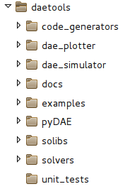
Fig. 5.1 DAE Tools folder structure.

5.1. Running tutorials

Start DAE Tools Tutorials program to try some examples:

• GNU/Linux:

  Run Applications/Development/DAE Tools Examples from the system menu

• Windows:

  Run i.e. Start/Programs/DAE Tools/daeExamples_2.2.0_py311 from the Start menu

Alternatively, run the following command from the command line (platform independent):

python -m daetools.examples.run_examples
or:
daeexamples

Note

daeexamples script is located in the Scripts folder (in Windows) or the bin folder (GNU/Linux) of the python installation. Typically, those locations are added to the PATH by the python installation.

The main window of DAE Tools Examples application is given in Fig. 5.2 while the output from the simulation run in Fig. 5.3. There, tutorials can be run, their source code inspected, and model reports generated. Model reports open in a new window of the system’s default web browser.

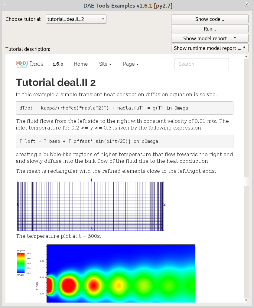
Fig. 5.2 DAE Tools Examples main window.

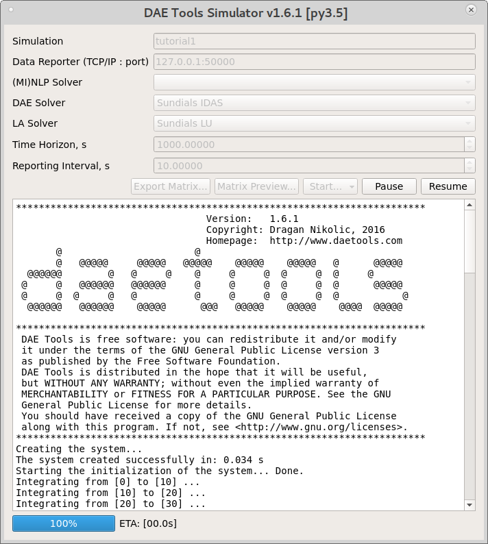
Fig. 5.3 A typical simulation output.

Tutorials can also be started from the shell:

cd .../daetools/examples

python tutorial1.py console
or:
python tutorial1.py gui

The sample output is given in Fig. 5.4:

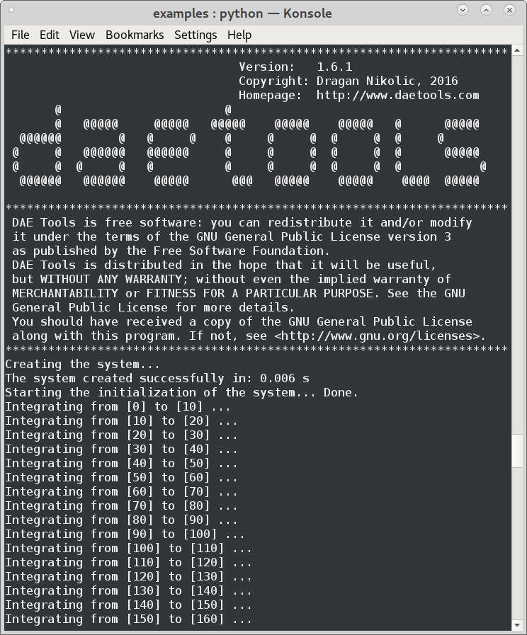
Fig. 5.4 Shell output from the simulation.

On GNU/Linux and Windows the DAE Plotter is started automatically. It can also be started manually:

• GNU/Linux:

  Run Applications/Development/DAE Tools Plotter from the system menu.

• Windows:

  Run i.e. Start/Programs/DAE Tools/daePlotter_2.2.0_py311 from the Start menu

Alternatively, run the following command from the command line (platform independent):

python -m daetools.dae_plotter.plotter
or:
daeplotter

Note

daeplotter script is located in the Scripts folder (in Windows) or the bin folder (GNU/Linux) of the python installation. Typically, those locations are added to the PATH by the python installation.

The DAE Tools Plotter main window should appear (given in Fig. 5.5)

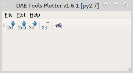
Fig. 5.5 DAE Tools Plotter main window.

5.2. Processing the results

DAE Tools provide a protocol for reporting the simulation results. It uses a concept of data reporter and data receiver interfaces. Data reporter interface is used by a simulation to send the data, while the data receiver interface is used to receive, store and provide the data to users. There are two types of data reporters: local (store data locally) and remote (send data to a server, i.e. via TCP/IP protocol).

There are three ways to obtain the results from the simulation:

• Through DAE Tools Plotter GUI

• Programmatically, using one of many different types of local data reporters

• Develop a custom user-defined data reporter by deriving from one of the available base classes (daeDataReporter_t, daeDataReporterLocal, daeDataReporterFile etc.)

5.2.1. DAE Tools Plotter

The simulation/optimisation results can be plotted using the DAE Tools Plotter application. Several types of plots are supported: Matplotlib-based 2D, animated 2D, auto-update 2D plots, user-defined plot, plot from the user-specified data, Mayavi 3D plot, and VTK file plot. After choosing a desired type, a Choose variable (given in Fig. 5.6) dialog appears where a variable to be plotted can be selected and information about domains specified - some domains should be fixed while leaving another free by selecting * from the list (to create a 2D plot one domain must remain free, while for a 3D plot two domains).

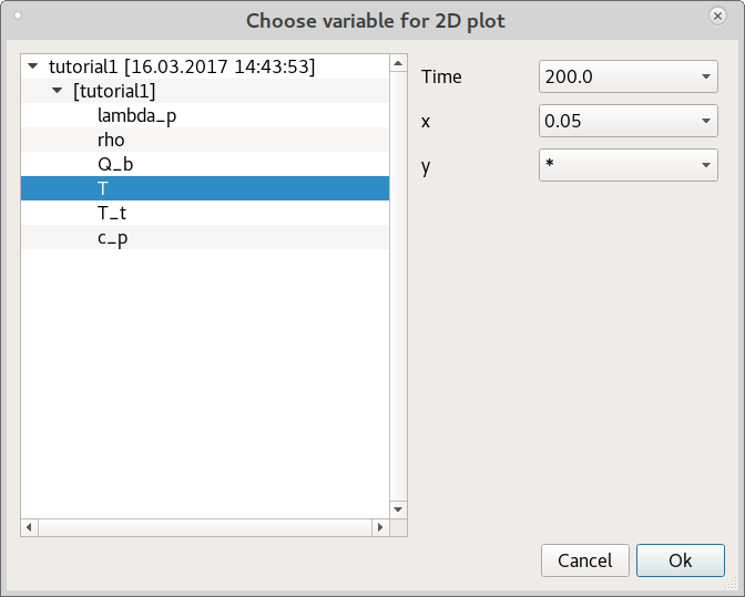
Fig. 5.6 Choose variable dialog for a 2D plot.

Typical 2D and 3D plots are given in Fig. 5.7 and Fig. 5.8.

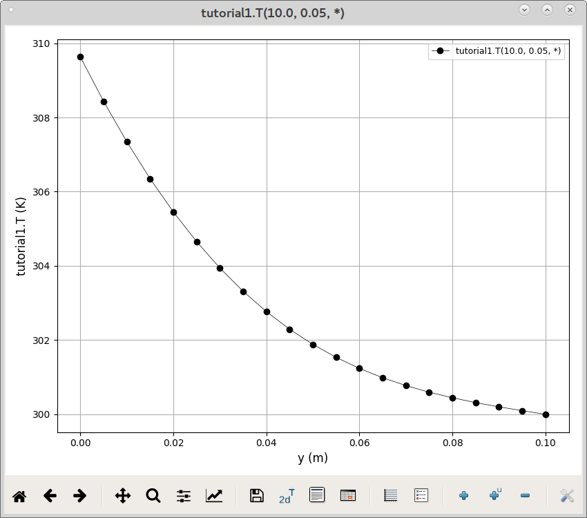
Fig. 5.7 Example 2D plot (produced by Matplotlib).

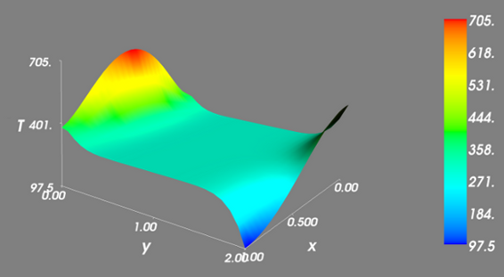
Fig. 5.8 Example 3D plot (produced by Mayavi2).

2D plots can be saved as templates (.pt files) which store the information in JSON format.

{
  "curves": [
      [
      "tutorial4.T",
      [
          -1
      ],
      [
          "*"
      ],
      "tutorial4.T(*)",
      {
          "color": "black",
          "linestyle": "-",
          "linewidth": 0.5,
          "marker": "o",
          "markeredgecolor": "black",
          "markerfacecolor": "black",
          "markersize": 6
      }
      ]
  ],
  "gridOn": true,
  "legendOn": true,
  "plotTitle": "",
  "updateInterval": 0,
  "windowTitle": "tutorial4.T(*)",
  "xlabel": "Time (s)",
  "xmax": 525.0,
  "xmax_policy": 0,
  "xmin": -25.0,
  "xmin_policy": 0,
  "xscale": "linear",
  "xtransform": 1.0,
  "ylabel": "T (K)",
  "ymax": 361.74772465755922,
  "ymax_policy": 1,
  "ymin": 279.2499308975365,
  "ymin_policy": 1,
  "yscale": "linear",
  "ytransform": 1.0,
}

5.2.2. Getting the results programmatically

There is a large number of available data reporters. Some of them are listed below.

• Data reporters that export the results to a specified file format:

  • Matlab .mat file (daeMatlabMATFileDataReporter)

  • Excell .xls file (daeExcelFileDataReporter)

  • JSON format (daeJSONFileDataReporter)

  • XML file (daeXMLFileDataReporter)

  • HDF5 file (daeHDF5FileDataReporter)

  • VTK file (daeVTKFileDataReporter)

• Other types of data reporters

  • Pandas dataset (daePandasDataReporter)

  • Quick matplotlib plots (daePlotDataReporter)

  • A container that delegates all calls to the contained data reporters; can contain one or more data reporters; useful to produce results in more than one format (daeDelegateDataReporter)

• Base-classes that can be used for development of custom data reporters:

  • daeDataReporterLocal (stores results internally; can be used for any type of processing)

  • daeNoOpDataReporter (stores results internally but does nothing with them)

  • daeDataReporterFile (saves the results into a file in the WriteDataToFile virtual member function)

  • daeBlackHoleDataReporter (does not store the results and does not process them; useful when the results are not needed)

5.3. Models

5.3.1. Developing a model

In DAE Tools models are developed by deriving a new class from the base model class (daeModel). The process consists of two steps:

1. Declaration of the model structure (parameters, variables, distribution domains, ports etc.):

   • In pyDAE declaration and instantiation in the __init__() function

   • In cDAE declaration as class data members and instantiation in the constructor

2. Specification of the model functionality (equations and state transition networks) in the DeclareEquations() function

An example model developed in pyDAE (using python programming language):

from daetools.pyDAE import *

class myModel(daeModel):
    def __init__(self, name, parent = None, description = ""):
        daeModel.__init__(self, name, parent, description)

        # Declaration/instantiation of domains, parameters, variables, ports, etc:
        self.m     = daeParameter("m",       kg,           self, "Mass of the copper plate")
        self.cp    = daeParameter("c_p",     J/(kg*K),     self, "Specific heat capacity of the plate")
        self.alpha = daeParameter("α", W/((m**2)*K), self, "Heat transfer coefficient")
        self.A     = daeParameter("A",       m**2,         self, "Area of the plate")
        self.Tsurr = daeParameter("T_surr",  K,            self, "Temperature of the surroundings")

        self.Qin   = daeVariable("Q_in",  power_t,       self, "Power of the heater")
        self.T     = daeVariable("T",     temperature_t, self, "Temperature of the plate")

    def DeclareEquations(self):
        # Specification of equations and state transitions:
        eq = self.CreateEquation("HeatBalance", "Integral heat balance equation")
        eq.Residual = self.m() * self.cp() * self.T.dt() - self.Qin() + self.alpha() * self.A() * (self.T() - self.Tsurr())

The same model developed in cDAE (using c++ programming language):

class myModel : public daeModel
{
public:
    // Declarations of domains, parameters, variables, ports, etc:
    daeParameter mass;
    daeParameter c_p;
    daeParameter alpha;
    daeParameter A;
    daeParameter T_surr;
    daeVariable  Q_in;
    daeVariable  T;

public:
    myModel(string strName, daeModel* pParent = NULL, string strDescription = "")
      : daeModel(strName, pParent, strDescription),

      // Instantiation of domains, parameters, variables, ports, etc:
      mass  ("m",       kg,            this, "Mass of the copper plate"),
      c_p   ("c_p",     J/(kg*K),      this, "Specific heat capacity of the plate"),
      alpha ("α", W/((m^2) * K), this, "Heat transfer coefficient"),
      A     ("A",       m ^ 2,         this, "Area of the plate"),
      T_surr("T_surr",  K,             this, "Temperature of the surroundings"),
      Q_in  ("Q_in",    power_t,       this, "Power of the heater"),
      T     ("T",       temperature_t, this, "Temperature of the plate")
    {
    }

    void DeclareEquations(void)
    {
        // Specification of equations and state transitions:
        daeEquation* eq = CreateEquation("HeatBalance", "Integral heat balance equation");
        eq->SetResidual( mass() * c_p() * T.dt() - Q_in() + alpha() * A() * (T() - T_surr()) );
    }
};

More information about developing models can be found in User Guide and pyCore.daeModel. Also, do not forget to have a look on Tutorials.

5.4. Simulation

5.4.1. Setting up a simulation

Definition of a simulation in DAE Tools requires the following steps:

1. Derivation of a new class from the base simulation class (daeSimulation)

   • Specification of a model to be simulated

   • Setting the values of parameters

   • Fixing the degrees of freedom by assigning the values to certain variables

   • Setting the initial conditions for differential variables

   • Setting the other variables’ information: initial guesses, absolute tolerances, etc

   • Specification of an operating procedure. It can be either a simple run for a specified period of time (default) or a complex one where various actions can be taken during the simulation

2. Specification of DAE and LA solvers

3. Specification of a data reporter and its connection

4. Setting a time horizon, reporting interval, etc

5. Initialisation of the DAE system

6. (Optionally) Saving a model report and/or a runtime model report (to inspect expanded equations etc)

7. Running the simulation

An example simulation developed in pyDAE:

class mySimulation(daeSimulation):
    def __init__(self):
        daeSimulation.__init__(self)

        # Set the model to simulate:
        self.m = myModel("myModel")

    def SetUpParametersAndDomains(self):
        # Set the parameters values:
        self.m.cp.SetValue(385 * J/(kg*K))
        self.m.m.SetValue(1 * kg)
        self.m.alpha.SetValue(200 * W/((m**2)*K))
        self.m.A.SetValue(0.1 * m**2)
        self.m.Tsurr.SetValue(283 * K)

    def SetUpVariables(self):
        # Set the degrees of freedom, initial conditions, initial guesses, etc.:
        self.m.Qin.AssignValue(1500 * W)
        self.m.T.SetInitialCondition(283 * K)

    def Run(self):
        # A custom operating procedure, if needed.
        # Here we use the default one:
        daeSimulation.Run(self)

The same simulation in cDAE:

class mySimulation : public daeSimulation
{
public:
    myModel m;

public:
    mySimulation(void) : m("myModel")
    {
        // Set the model to simulate:
        SetModel(&m);
    }

public:
    void SetUpParametersAndDomains(void)
    {
        // Set the parameters values:
        model.c_p.SetValue(385 * J/(kg*K));
        model.mass.SetValue(1 * kg);
        model.alpha.SetValue(200 * W/((m^2)*K));
        model.A.SetValue(0.1 * (m^2));
        model.T_surr.SetValue(283 * K);
    }

    void SetUpVariables(void)
    {
        // Set the degrees of freedom, initial conditions, initial guesses, etc.:
        model.Q_in.AssignValue(1500 * W);
        model.T.SetInitialCondition(283 * K);
    }

    void Run(void)
    {
        // A custom operating procedure, if needed.
        // Here we use the default one:
        daeSimulation::Run();
    }
};

Simulations in pyDAE can be set-up to run in two modes:

1. From the PyQt4 graphical user interface (pyDAE only):

   Here the default log, and data reporter objects will be used, while the user can choose DAE and LA solvers and specify time horizon and reporting interval.

   # Import modules
   import sys
   from time import localtime, strftime
   from PyQt4 import QtCore, QtGui
   
   # Create QtApplication object
   app = QtGui.QApplication(sys.argv)
   
   # Create simulation object
   sim = mySimulation()
   
   # Report ALL variables in the model
   sim.m.SetReportingOn(True)
   
   # Show the daeSimulator window to choose the other information needed for simulation
   simulator  = daeSimulator(app, simulation=sim)
   simulator.show()
   
   # Execute applications main loop
   app.exec_()
   

2. From the shell:

   In pyDAE:

   # Import modules
   import sys
   from time import localtime, strftime
   
   # Create Log, Solver, DataReporter and Simulation object
   log          = daeStdOutLog()
   solver       = daeIDAS()
   datareporter = daeTCPIPDataReporter()
   simulation   = mySimulation()
   
   # Report ALL variables in the model
   simulation.m.SetReportingOn(True)
   
   # Set the time horizon (1000 seconds) and the reporting interval (10 seconds)
   simulation.SetReportingInterval(10)
   simulation.SetTimeHorizon(1000)
   
   # Connect data reporter
   # (use the default TCP/IP connection settings: localhost and 50000 port)
   simName = simulation.m.Name + strftime(" [m.%Y %H:%M:%S]", localtime())
   if(datareporter.Connect("", simName) == False):
       sys.exit()
   
   # Initialize the simulation
   simulation.Initialize(solver, datareporter, log)
   
   # Solve at time = 0 (initialization)
   simulation.SolveInitial()
   
   # Run
   simulation.Run()
   
   # Clean up
   simulation.Finalize()
   

   In cDAE:

   // Create Log, Solver, DataReporter and Simulation object
   boost::scoped_ptr<daeSimulation_t>    pSimulation(new mySimulation());
   boost::scoped_ptr<daeDataReporter_t>  pDataReporter(daeCreateTCPIPDataReporter());
   boost::scoped_ptr<daeIDASolver>       pDAESolver(daeCreateIDASolver());
   boost::scoped_ptr<daeLog_t>           pLog(daeCreateStdOutLog());
   
   // Report ALL variables in the model
   pSimulation->GetModel()->SetReportingOn(true);
   
   // Set the time horizon (1000 seconds) and the reporting interval (10 seconds)
   pSimulation->SetReportingInterval(10);
   pSimulation->SetTimeHorizon(1000);
   
   // Connect data reporter
   // (use the default TCP/IP connection settings: localhost and 50000 port)
   string strName = pSimulation->GetModel()->GetName();
   if(!pDataReporter->Connect("", strName))
       return;
   
   // Initialize the simulation
   pSimulation->Initialize(pDAESolver.get(), pDataReporter.get(), pLog.get());
   
   // Solve at time = 0 (initialization)
   pSimulation->SolveInitial();
   
   // Run
   pSimulation->Run();
   
   // Clean up
   pSimulation->Finalize();
   

5.4.2. Running a simulation

Simulations are started by executing the following shell commands:

cd "directory where simulation file is located"
python mySimulation.py

5.5. Optimisation

5.5.1. Setting up an optimisation

To define an optimisation problem it is first necessary to develop a model of the process and to define a simulation (as explained above). Having done these tasks (working model and simulation) the optimisation in DAE Tools can be defined by specifying the objective function, optimisation variables and optimisation constraints. It is intentionally chosen to keep simulation and optimisation tightly coupled. The optimisation problem should be specified in the function SetUpOptimization().

Definition of an optimisation in DAE Tools requires the following steps:

1. Specification of the objective function

   • Objective function is defined by specifying its residual (similarly to specifying an equation residual); Internally the framework will create a new variable (V_obj) and a new equation (F_obj).

2. Specification of optimisation variables

   • The optimisation variables have to be already defined in the model and their values assigned in the simulation; they can be either non-distributed or distributed.

   • Specify a type of optimisation variable values. The variables can be continuous (floating point values in the given range), integer (set of integer values in the given range) or binary (integer value: 0 or 1).

   • Specify the starting point (within the range)

3. Specification of optimisation constraints

   • Two types of constraints exist in DAE Tools: equality and inequality constraints To define an equality constraint its residual and the value has to be specified; To define an inequality constraint its residual, the lower and upper bounds have to be specified; Internally the framework will create a new variable (V_constraint[N]) and a new equation (F_constraint[N]) for each defined constraint, where N is the ordinal number of the constraint.

4. Specification of a NLP/MINLP solver

   • Currently BONMIN MINLP solver and IPOPT and NLOPT solvers are supported (the BONMIN solver internally uses IPOPT to solve NLP problems)

5. Specification of DAE and LA solvers

6. Specification of a data reporter and its connection

7. Setting a time horizon, reporting interval, etc

8. Setting the options of the (MI)NLP solver

9. Initialisation of the optimisation

10. Running the optimisation

SetUpOptimization() function should be declared in the simulation class:

In pyDAE:

class mySimulation(daeSimulation):
    ...

    def SetUpOptimization(self):
        # Declarations of the obj. function, opt. variables and constraints:
         ...

In cDAE:

class mySimulation : public daeSimulation
{
    ...

    void SetUpOptimization(void)
    {
        // Declarations of the obj. function, opt. variables and constraints:
    }
};

Optimisations, like simulations can be set-up to run in two modes:

1. From the PyQt4 graphical user interface (pyDAE only)

   Here the default log, and data reporter objects will be used, while the user can choose NLP, DAE and LA solvers and specify time horizon and reporting interval:

   # Import modules
   import sys
   from time import localtime, strftime
   from PyQt4 import QtCore, QtGui
   
   # Create QtApplication object
   app = QtGui.QApplication(sys.argv)
   
   # Create simulation object
   sim = mySimulation()
   nlp = daeBONMIN()
   
   # Report ALL variables in the model
   sim.m.SetReportingOn(True)
   
   # Show the daeSimulator window to choose the other information needed for optimisation
   simulator = daeSimulator(app, simulation=sim, nlpsolver=nlp)
   simulator.show()
   
   # Execute applications main loop
   app.exec_()
   

2. From the shell:

   In pyDAE:

   # Create Log, NLPSolver, DAESolver, DataReporter, Simulation and Optimization objects
   log          = daePythonStdOutLog()
   daesolver    = daeIDAS()
   nlpsolver    = daeIPOPT()
   datareporter = daeTCPIPDataReporter()
   simulation   = mySimulation()
   optimization = daeOptimization()
   
   # Enable reporting of all variables
   simulation.m.SetReportingOn(True)
   
   # Set the time horizon and the reporting interval
   simulation.ReportingInterval = 10
   simulation.TimeHorizon = 100
   
   # Connect data reporter
   simName = simulation.m.Name + strftime(" [m.%Y %H:%M:%S]", localtime())
   if(datareporter.Connect("", simName) == False):
       sys.exit()
   
   # Initialise the optimisation
   optimization.Initialize(simulation, nlpsolver, daesolver, datareporter, log)
   
   # Run
   optimization.Run()
   
   # Clean up
   optimization.Finalize()
   

   In cDAE:

   // Create Log, NLPSolver, DAESolver, DataReporter, Simulation and Optimization objects
   boost::scoped_ptr<daeSimulation_t>        pSimulation(new mySimulation());
   boost::scoped_ptr<daeDataReporter_t>      pDataReporter(daeCreateTCPIPDataReporter());
   boost::scoped_ptr<daeIDASolver>           pDAESolver(daeCreateIDASolver());
   boost::scoped_ptr<daeLog_t>               pLog(daeCreateStdOutLog());
   boost::scoped_ptr<daeNLPSolver_t>         pNLPSolver(new daeIPOPTSolver());
   boost::scoped_ptr<daeOptimization_t>      pOptimization(new daeOptimization());
   
   // Report ALL variables in the model
   pSimulation->GetModel()->SetReportingOn(true);
   
   // Set the time horizon and the reporting interval
   pSimulation->SetReportingInterval(10);
   pSimulation->SetTimeHorizon(100);
   
   // Connect data reporter
   string strName = pSimulation->GetModel()->GetName();
   if(!pDataReporter->Connect("", strName))
       return;
   
   // Initialise the optimisation
   pOptimization->Initialize(pSimulation.get(),
                             pNLPSolver.get(),
                             pDAESolver.get(),
                             pDataReporter.get(),
                             pLog.get());
   
   // Run
   pOptimization.Run();
   
   // Clean up
   pOptimization.Finalize();
   

More information about simulation can be found in User Guide and daeOptimization. Also, do not forget to have a look on Tutorials.

5.5.2. Starting an optimisation

Starting the optimisation problems is analogous to running a simulation.