6. User Guide

6.1. Importing DAE Tools modules

DAE Tools are loaded by importing daetools.pyDAE Python module:

from daetools.pyDAE import *

This sets the python sys.path for importing the platform dependent extension modules (i.e. …/daetools/pyDAE/Windows_win32_py34 and …/daetools/solvers/Windows_win32_py34 in Windows, …/daetools/pyDAE/Linux_x86_64_py34 and …/daetools/solvers/Linux_x86_64_py34 in GNU/Linux), import all symbols from all pyDAE modules: pyCore, pyActivity, pyDataReporting, pyIDAS, pyUnits and import some platform independent modules: logs, variable_types, hr_upwind_scheme, simulator, simulation_explorer, simulation_inspector, thermo_packages.

Alternatively, the daetools.pyDAE module can be imported and classes from the pyDAE extension modules accessed using the fully qualified names. For instance:

import daetools.pyDAE

model = daetools.pyDAE.pyCore.daeModel("name")

Once the daetools.pyDAE module is loaded, the other modules (such as third party linear solvers, optimisation solvers etc.) can be imported. Since domains, parameters and variables in DAE Tools have a numerical value in terms of a unit of measurement (quantity) the modules containing definitions of units and variable types must be imported:

from daetools.pyDAE.variable_types import length_t, area_t, volume_t
from daetools.pyDAE.pyUnits import m, kg, s, K, Pa, J, W

The complete list of units and variable types can be found in variable_types and pyUnits modules.

6.2. Developing models

DAE Tools models are developed by deriving a class from the base daeModel:

class myModel(daeModel):
    def __init__(self, name, parent = None, description = ""):
        daeModel.__init__(self, name, parent, description)

        # Declaration/instantiation of domains, parameters, variables, ports, etc:
        ...

    def DeclareEquations(self):
        # Declaration of equations, state transition networks etc.:
        ...

Every model definition requires specification of the model structure and its functionality in two phases:

1. Declaring the model structure (domains, parameters, variables, ports, components etc.) in the __init__() function:

   In DAE Tools the model specification is separated from the activities that can be performed on the model. This way, based on a single model definition different simulation scenarios can be developed. Thus, all objects are specified in two stages:

   • Declaration in the __init__() function

   • Initialisation of domains and parameters in SetUpParametersAndDomains() and variables in SetUpVariables() function.

   Therefore, parameters, domains and variables are only declared here, while their initialisation (i.e. setting parameter values or initial conditions) is postponed and performed in the simulation class.

   All objects must be stored in the model since the base daeModel class keeps only week references to them:

   def __init__(self, name, parent = None, description = ""):
       self.domain    = daeDomain(...)
       self.parameter = daeParameter(...)
       self.variable  = daeVariable(...)
       ... etc.
   

   and not:

   def __init__(self, name, parent = None, description = ""):
       domain    = daeDomain(...)
       parameter = daeParameter(...)
       variable  = daeVariable(...)
       ... etc.
   

   because at the exit from the __init__() function the objects will go out of scope and get destroyed. However, the underlying c++ model still holds pointers which eventually results in the segmentation fault.

2. Specification of the model functionality (equations, state transition networks, and OnEvent and OnCondition actions) in the DeclareEquations() function.

   Nota bene: This function is never called directly by the user and will be called automatically by the framework.

   Initialisation of the simulation object is carried out in several phases. At the point when this function is called by the framework, the model parameters, domains, variables etc. are fully initialised. Therefore, it is safe to obtain the values of parameters or domain points and use them to create equations at the run-time.

   Nota bene: However, the variable values are obviously not available at this moment (they get initialised at the later stage) and using the variable values during the model specification phase is not allowed.

A simplest DAE Tools model with a description of all steps/tasks necessary to develop a model can be found in the What’s the time? (AKA: Hello world!) tutorial (whats_the_time.py).

6.2.1. Parameters

Parameters are time invariant quantities that do not change during a simulation. Usually a good choice what should be a parameter is a physical constant, number of discretisation points in a domain etc.

Again, parameters are defined in two phases:

• Declaration in the __init__() function

• Initialisation (by setting its value) in the SetUpParametersAndDomains() function

6.2.1.1. Declaring parameters

Parameters are declared in the __init__() function:

self.myParam = daeParameter("myParam", units, parentModel, "description")

Parameters can also be distributed on domains:

self.myParam = daeParameter("myParam", units, parentModel, "description")
self.myParam.DistributeOnDomain(myDomain)

# Or simply:
self.myParam = daeParameter("myParam", units, parentModel, "description", [myDomain])

6.2.1.2. Initialising parameters

Parameters are initialised in the SetUpParametersAndDomains() function:

# Ordinary parameters:
myParam.SetValue(value)

# Distributed parameters (one-dimensional):
for i in range(myDomain.NumberOfPoints):
    myParam.SetValue(i, value)

where value can be either a floating point number or the quantity object (i.e. 1.34 * W/(m*K)). If the simple floats are used it is assumed that they represent values with the same units as in the parameter definition.

Nota bene

DAE Tools (as it is the case in C/C++ and Python) use zero-based arrays in which the initial element of a sequence is assigned the index 0, rather than 1.

In addition, all values in a distributed parameter can be set in a single call:

myParam.SetValues(values)

where values is a numpy array of floats/quantity objects.

6.2.1.3. Using parameters

Model equations consist of mathematical operations and functions that operate on adouble and adouble_array objects. They contain information about the functions and operands in the Node attribute. adouble objects contain the values of parameters and variables while adouble_array objects contain arrays of values.

1. A parameter value can be obtained using the __call__() function (operator ()) which returns the adouble object. For instance, the equation:

   \[myVar = myParam + 15\]

   is specified in the following (acausal) way:

   # Notation:
   #  - eq is a daeEquation object created using the model.CreateEquation(...) function
   #  - myParam is an ordinary daeParameter object (not distributed)
   #  - myVar is an ordinary daeVariable (not distributed)
   
   eq.Residual = myVar() - (myParam() + 15)
   

   The same function is used for distributed parameters. For instance, the equation:

   \[myVar(i) = myParam(i) + 15; \forall i \in [0, n_d - 1]\]

   is given as:

   # Notation:
   #  - myDomain is daeDomain object
   #  - eq is a daeEquation object distributed on myDomain
   #  - i is daeDistributedEquationDomainInfo object (used to iterate through the domain points)
   #  - myParam is daeParameter object distributed on myDomain
   #  - myVar is daeVariable object distributed on myDomain
   i = eq.DistributeOnDomain(myDomain, eClosedClosed)
   eq.Residual = myVar(i) - (myParam(i) + 15)
   

   This code translates into a set of n algebraic equations.

   Obviously, a parameter can be distributed on more than one domain. The equation:

   \[myVar(d_1,d_2) = myParam(d_1,d_2) + 15; \forall d_1 \in [0, n_{d1} - 1], \forall d_2 \in [0, n_{d2} - 1]\]

   is specified as:

   # Notation:
   #  - myDomain1, myDomain2 are daeDomain objects
   #  - eq is a daeEquation object distributed on the domains myDomain1 and myDomain2
   #  - i1, i2 are daeDistributedEquationDomainInfo objects (used to iterate through the domain points)
   #  - myParam is daeParameter object distributed on myDomain1 and myDomain2
   #  - myVar is daeVariable object distributed on myDomain1 and myDomain2
   i1 = eq.DistributeOnDomain(myDomain1, eClosedClosed)
   i2 = eq.DistributeOnDomain(myDomain2, eClosedClosed)
   eq.Residual = myVar(i1,i2) - (myParam(i1,i2) + 15)
   

2. An array of parameter values can be obtained using the function array() which returns the adouble_array object. The function accepts the following type of arguments:

   • integers (to select a single index from a domain); a special case is index -1 that returns the last point in the domain)

   • python list (to select a list of indexes from a domain)

   • python slice (to select a portion of indexes from a domain: startIndex, endIindex, step)

   • character ‘*’ or an empty python list [] (to select all points from a domain)

   For example, the equation:

   \[myVar = \sum myParam(0, *)\]

   can be written in two ways:

   # Notation:
   #  - myDomain1, myDomain2 are daeDomain objects
   #  - n1, n2 are the number of points in myDomain1 and myDomain2 domains
   #  - eq is daeEquation objects
   #  - mySum is daeVariable object
   #  - myParam is daeParameter object distributed on myDomain1 and myDomain2 domains
   #  - values is the adouble_array object
   
   # An array contains myParam values for:
   #  - the first point in the domain myDomain1
   #  - all points from the domain myDomain2
   # The expressions below are equivalent:
   values = myParam.array(0, '*')
   values = myParam.array(0, [])
   
   eq.Residual = mySum() - Sum(values)
   

   The code translates into:

   \[mySum = myParam(0,0) + myParam(0,1) + ... + myParam(0,n_2 - 1)\]

   where n2 is the number of points in the domain myDomain2.

   In addition, the function supports advanced indexing. For instance, the equation:

   \[myVar = \sum myParam([0,1,2], [even\_points\_in\_myDomain2])\]

   is defined as:

   # An array contains the following values from myParam:
   #  - the first three points in the domain myDomain1
   #  - all even points from the domain myDomain2
   values = myParam.array([0,1,2], slice(0, myDomain2.NumberOfPoints, 2))
   
   eq.Residual = mySum() - Sum(values)
   

   The code translates into:

   \[\begin{split}mySum = & myParam(0,0) + myParam(0,2) + myParam(0,4) + ... + myParam(0, n_2 - 1) + \\ & myParam(1,0) + myParam(1,2) + myParam(1,4) + ... + myParam(1, n_2 - 1) + \\ & myParam(2,0) + myParam(2,2) + myParam(2,4) + ... + myParam(2, n_2 - 1)\end{split}\]

The property npyValues contains the parameter values as a numpy multi-dimensional array (with ‘numpy.float’ data type).

Notate bene

The functions __call__() and array() return adouble and adouble_array objects, respectively and does not contain values. They are only used to specify equations’ residual expressions which are stored in their pyCore.adouble.Node / pyCore.adouble_array.Node properties.

Other functions (such as npyValues and GetValue()) can be used to access the values data during the simulation.

All above stands for similar functions in daeDomain and daeVariable classes.

More information about parameters can be found in the API reference daeParameter and in Tutorials.

6.2.2. Variable types

Variable types describe variables and contain the information such as:

• Name: string

• Units: unit object

• LowerBound: float

• UpperBound: float

• InitialGuess: float

• AbsoluteTolerance: float

• ValueConstraint: enumeration daeeVariableValueConstraint

Declaration of variable types is commonly done outside of the model definition (in the module scope):

# Temperature type with units Kelvin, limits 100-1000K, the default value 273K and the absolute tolerance 1E-5
typeTemperature = daeVariableType("Temperature", K, 100, 1000, 273, 1E-5, constraint)

where the argument constraint specifies the value constraint and can be one of:

• eNoConstraint (default)

• eValueGTEQ: imposes >= 0 constraint

• eValueLTEQ: imposes <= 0 constraint

• eValueGT: imposes > 0 constraint

• eValueLT: imposes < 0 constraint

6.2.3. Distribution domains

Domains in DAE Tools are used to to create simple arrays of variables, parameters, equations and ports and their distributions in space. They can define uniform (the default) or non-uniform grids (user-specified) and are defined in two phases:

• Declaring a domain in the model

• Initialising it in the simulation

6.2.3.1. Declaring domains

Domains are declared in the __init__() function:

self.myDomain = daeDomain("myDomain", parentModel, units, "description")

6.2.3.2. Initialising domains

Domains are initialised in the SetUpParametersAndDomains() function. Simple arrays are defined using the function CreateArray():

# Array of N elements
myDomain.CreateArray(N)

while the domains distributed on a structured grid using the function CreateStructuredGrid():

# Uniform structured grid with N elements and bounds [lowerBound, upperBound]
myDomain.CreateStructuredGrid(N, lowerBound, upperBound)

where the lower and upper bounds are the floating point values or quantity objects. If the floats are used it is assumed that they contain values with the same units as in the domain definition. Using the quantities is advised (to avoid problems when the domain units change).

# Uniform structured grid with 10 elements and bounds [0,1] in centimeters:
myDomain.CreateStructuredGrid(10, 0.0 * cm, 1.0 * cm)

Nota bene

Structured grids with N elements contain N+1 points.

It is also possible to create an unstructured grid (for use in Finite Element models). However, their structure is an implementation detail (i.e. as in deal.II).

In certain situations it is desired to have a non-uniform distribution of the points within the given interval, defined by the lower and upper bounds. In these cases, a non-uniform structured grid can be specified using the attribute Points which contains the list of the points and that can be manipulated by the user:

# First create a structured grid domain
myDomain.CreateStructuredGrid(10, 0.0, 1.0)

# The original 11 points are: [0.0, 0.1, 0.2, 0.3, 0.4, 0.5, 0.6, 0.7, 0.8, 0.9, 1.0]
# If the system is stiff at the beginning of the domain more points can be placed there
myDomain.Points = [0.0, 0.05, 0.10, 0.15, 0.20, 0.25, 0.30, 0.35, 0.40, 0.60, 1.00]

The effect of uniform and non-uniform grids is given in Fig. 6.1 (a simple heat conduction problem from the Tutorial 3 has been served as a basis for comparison). Here, there are three cases:

• Black line: the analytic solution

• Blue line (10 intervals): uniform grid - a very rough prediction

• Red line (10 intervals): non-uniform grid - more points at the beginning of the domain

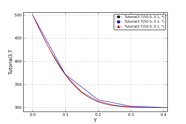
Fig. 6.1 Effect of uniform and non-uniform grids on numerical solution (zoomed to the first 5 points)

More precise results are obtained by using denser grid at the beginning of the interval.

6.2.3.3. Using domains

The functions __call__() (operator ()) and __getitem__() (operator []) are used to return the adouble object with the value of the point at the specified index within the domain. Both functions have the same functionality. For instance, the equation:

\[myVar = myDomain[5]\]

is specified in the following way:

# Notation:
#  - eq is a daeEquation object
#  - myDomain is daeDomain object
#  - myVar is daeVariable object
eq.Residual = myVar() - myDomain[5]

The function array() returns the adouble_array object with an array of points. It accepts the same type of arguments as explained in the section Using parameters.

The property Points contains a list of the points in the domain.

Nota bene

The functions __call__(), __getitem__() and array() can only be used to build equations’ residual expressions. On the other hand, the attribute Points can be used at any point.

More information about domains can be found in the API reference daeDomain and in Tutorials.

6.2.4. Variables

Variables define time varying quantities that change during a simulation and can be:

• Algebraic

• Differential

• Assigned (that is their value is assigned by fixing the number of degrees of freedom - DOF)

They are defined in two phases:

• Declaring a variable in the model

• Initialising it, if required (by assigning its value or setting an initial condition) in the simulation

6.2.4.1. Declaring variables

Variables are declared in the __init__() function:

# Ordinary variables:
self.myVar = daeVariable("myVar", variableType, parentModel, "description")

# Distributed variables:
self.myVar = daeVariable("myVar", variableType, parentModel, "description")
self.myVar.DistributeOnDomain(myDomain)
# or simply:
self.myVar = daeVariable("myVar", variableType, parentModel, "description", [myDomain])

6.2.4.2. Initialising variables

Variables are initialised in the SetUpVariables() function:

• The function AssignValue() is used to specify degrees of freedom:

  myVar.AssignValue(value)
  
  # If the variable is distributed:
  for i in range(myDomain.NumberOfPoints):
      myVar.AssignValue(i, value)
  
  # In addition, all values can be specified in a single call using a numpy array:
  myVar.AssignValues(values)
  

  where the argument value can be either a floating point number or the quantity object (i.e. 1.34 * W/(m*K)), and values is a numpy array of floats or quantity objects. If the simple floats are used it is assumed that they represent values with the same units as in the variable type definition.

  The functions ReAssignValue() and ReAssignValues() are used in a schedule during a simulation (in the function Run()) to re-assign the variable with the new value(s).

• The function SetInitialCondition() is used to set initial conditions:

  myVar.SetInitialCondition(value)
  
  # If the variable is distributed:
  for i in range(myDomain.NumberOfPoints):
      myVar.SetInitialCondition(i, value)
  
  # In addition, all values can be specified in a single call using a numpy array:
  myVar.SetInitialConditions(values)
  

  The functions ReSetInitialCondition() and ReSetInitialConditions() are used in a schedule during a simulation (in the function Run()) to re-initialise the variable with the new value(s).

• The function SetAbsoluteTolerances() is used to set absolute tolerances:

  myVar.SetAbsoluteTolerances(1E-5)
  

• The function SetInitialGuess() is used to set initial guesses:

  myVar.SetInitialGuess(value)
  
  # If the variable is distributed:
  for i in range(0, myDomain.NumberOfPoints):
      myVar.SetInitialGuess(i, value)
  
  # In addition, all values can be specified in a single call using a numpy array:
  myVar.SetInitialGuesses(values)
  

6.2.4.3. Using variables

The functions __call__() and array() are used to get a value or an array of values (for use in model equations only). They accept the same type of arguments as explained in the section Using parameters. In addition, the following functions are used to get derivatives:

1. The function dt() is used to get a time derivative of an ordinary variable. For instance, the equation:

   \[{ d(myVar) \over {d}{t} } = 1\]

   is given as:

   # Notation:
   #  - eq is a daeEquation object
   #  - myVar is an ordinary daeVariable
   eq.Residual = dt(myVar()) - 1.0
   

   The same function is used for distributed variables. For example, the equation:

   \[{d(myVar(i)) \over dt} = 1; \forall i \in [0, n]\]

   is written as:

   # Notation:
   #  - myDomain is daeDomain object
   #  - n is the number of points in myDomain
   #  - eq is a daeEquation object distributed on myDomain
   #  - d1,d2 are objects used to iterate through the domain points
   #  - myVar is daeVariable object distributed on myDomain
   d = eq.DistributeOnDomain(myDomain, eClosedClosed)
   eq.Residual = dt(myVar(d)) - 1.0
   

   For variables that are distributed on more than one domain, the equation:

   \[{d(myVar(d_1, d_2)) \over dt} = 1; \forall d_1 \in [0, n_1], \forall d_2 \in [0, n_2]\]

   is specified as:

   # Notation:
   #  - myDomain1, myDomain2 are daeDomain objects
   #  - n1 is the number of points in myDomain1
   #  - n2 is the number of points in myDomain2
   #  - eq is a daeEquation object distributed on the domains myDomain1 and myDomain2
   #  - d is daeDEDI object (used to iterate through the domain points)
   #  - myVar is daeVariable object distributed on myDomain1 and myDomain2
   d1 = eq.DistributeOnDomain(myDomain1, eClosedClosed)
   d2 = eq.DistributeOnDomain(myDomain2, eClosedClosed)
   eq.Residual = dt(myVar(d1,d2)) - 1.0
   

   The code translates into a set of n1 x n2 equations.

   The function dt_array() is used to get an array of time derivatives. It accepts the same type of arguments as explained in the section Using parameters.

2. The functions d() and d2() are used to get a partial derivative of distributed variables. For instance, the equation:

   \[{\partial myVar(d) \over \partial myDomain} = 1.0; \forall d \in [0, n]\]

   is written as:

   # Notation:
   #  - myDomain is daeDomain object
   #  - n is the number of points in myDomain
   #  - eq is a daeEquation object distributed on myDomain
   #  - d is daeDEDI object (used to iterate through the domain points)
   #  - myVar is daeVariable object distributed on myDomain
   d = eq.DistributeOnDomain(myDomain, eClosedClosed)
   eq.Residual = d(myVar(d), myDomain, discretizationMethod=eCFDM, options={}) - 1.0
   
   # since the defaults are eCFDM and an empty options dictionary the above is equivalent to:
   eq.Residual = d(myVar(d), myDomain) - 1.0
   

   The default discretisation method is center finite difference method (eCFDM`) and the default discretisation order is 2 and can be specified in the options dictionary: options[“DiscretizationOrder”] = integer. At the moment, only the finite difference discretisation methods are supported by default (but the finite volume and finite elements implementations are available using the third party libraries):

   • Center finite difference method (eCFDM)

   • Backward finite difference method (eBFDM)

   • Forward finite difference method (eFFDM)

   The functions d_array() and d2_array() are used to get an array of partial derivatives. They accept the same type of arguments as explained in the section Using parameters.

The property npyValues contains the variable values as a numpy multi-dimensional array (with numpy.float data type). The functions SetValue() and GetValue() / GetQuantity() are used to get/set the variable value as a floating point number or the quantity object.

Nota bene

The functions __call__(), dt(), d(), d2(), array(), dt_array(), d_array() and d2_array() can only be used to build equations’ residual expressions. On the other hand, the functions GetValue, SetValue and npyValues can be used to access the variable data at any point.

More information about variables can be found in the API reference daeVariable and in Tutorials.

6.2.5. Ports

Ports define connection points between model instances for exchange of continuous quantities. Like models, they can contain domains, parameters and variables.

New type of ports are defined by deriving a class from the base daePort:

class myPort(daePort):
    def __init__(self, name, parent = None, description = ""):
        daePort.__init__(self, name, type, parent, description)

        # Declaration/instantiation of domains, parameters and variables
        ...

The port structure (domains, parameters and variables) is declared in the __init__() function. The same rules apply as described in the section Developing models. Two ports are connected using the ConnectPorts() function. Ports are instantiated as inlet or outlet type in the __init__() function:

self.myPort = daePort("myPort", eInletPort, parentModel, "description")

6.2.6. Event ports

Event ports define connection points between model instances for exchange of discrete messages/events. Events can be triggered manually (using the SendEvent() function) or when a specified condition is satisfied. The main difference between event and ordinary ports is that the former allow a discrete communication between models while the latter allow a continuous exchange of information.

Messages are floating point values that can be used by a recipient. Upon a reception of an event, a set of actions are executed. The actions are specified in the ON_EVENT() function. The events received by an event port can be recorded by setting the boolean RecordEvents property to True and retrieved using the Events property.

Two event ports are connected using the ConnectEventPorts() function. A single outlet event port can be connected to unlimited number of inlet event ports. Event ports are instantiated in the __init__() function:

self.myEventPort = daeEventPort("myEventPort", eOutletPort, parentModel, "description")

6.2.7. Equations

Model equations are specified in an implicit (acausal) form. They can be continuous or discontinuous and distributed on one or more domains. Equations can be distributed on a whole domain, on a portion of it or even on a single point (i.e. equations for boundary conditions).

6.2.7.1. Declaring equations

Equations are declared in the DeclareEquations() function:

# Ordinary equation:
eq = model.CreateEquation("MyEquation", "description")

# Distributed equation (on the whole domain, including the boundaries):
eq = model.CreateEquation("MyEquation")
d = eq.DistributeOnDomain(myDomain, eClosedClosed)

Currently, the following options for distributing equations are available:

• Distributed on a closed (whole) domain: \(x \in [x_0, x_n]\)

• Distributed on a left open domain: \(x \in (x_0, x_n]\)

• Distributed on a right open domain: \(x \in [x_0, x_n)\)

• Distributed on a domain open on both sides: \(x \in (x_0, x_n)\)

• Distributed on the lower bound: \(x \in \{ x_0 \}\)

• Distributed on the upper bound: \(x \in \{ x_n \}\)

• Distributed on a given set of points within a domain: i.e. \(x \in \{ x_0, x_3, x_7, x_8 \}\)

where \(x_0\) represents the lower bound and \(x_n\) the upper bound of the domain.

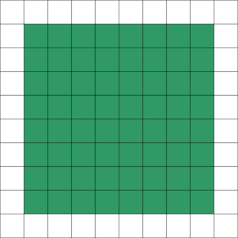
An overview of available options is given in the table below. The examples are given for an equation distributed on two domains: x and y. Green squares represent portions of a domain included in the distributed equation, while white squares represent excluded portions.

x = eClosedClosed; y = eClosedClosed \(x \in [x_0, x_n], y \in [y_0, y_n]\)	x = eOpenOpen; y = eOpenOpen \(x \in ( x_0, x_n ), y \in ( y_0, y_n )\)
x = eClosedClosed; y = eOpenOpen \(x \in [x_0, x_n], y \in ( y_0, y_n )\)	x = eClosedClosed; y = eOpenClosed \(x \in [x_0, x_n], y \in ( y_0, y_n ]\)
x = eLowerBound; y = eClosedOpen \(x = x_0, y \in [ y_0, y_n )\)	x = eLowerBound; y = eClosedClosed \(x = x_0, y \in [y_0, y_n]\)
x = eUpperBound; y = eClosedClosed \(x = x_n, y \in [y_0, y_n]\)	x = eLowerBound; y = eUpperBound \(x = x_0, y = y_n\)

6.2.7.2. Defining equations

Equations in DAE Tools are specified in implicit (acausal) form as residual expressions. For instance, a residual for an ordinary equation:

\[{\partial V_{14} \over \partial t} + {V_1 \over V_{14} + 2.5} + sin(3.14 \cdot V_3) = 0\]

is specified as:

# Notation:
#  - V1, V3, V14 are ordinary variables
eq.Residual = dt(V14()) + V1() / (V14() + 2.5) + sin(3.14 * V3())

while a distributed equation:

\[{\partial V_{14}(x,y)) \over \partial t} + {V_1 \over V_{14}(x,y) + 2.5} + sin(3.14 \cdot V_3(x,y)) = 0; \forall x \in [0, nx], \forall y \in (0, ny)\]

is given as:

# Notation:
#  - V1 is an ordinary variable
#  - V3 and V14 are variables distributed on domains x and y
eq = model.CreateEquation("MyEquation")
dx = eq.DistributeOnDomain(x, eClosedClosed)
dy = eq.DistributeOnDomain(y, eOpenOpen)
eq.Residual = dt(V14(dx,dy)) + V1() / ( V14(dx,dy) + 2.5) + sin(3.14 * V3(dx,dy) )

where dx and dy are daeDEDI (which is short for daeDistributedEquationDomainInfo) objects. These objects are used internally by the framework to iterate over the domain points when generating a set of equations from a distributed equation. Therefore, the equation above is equivalent to:

# Notation:
#  - V1 is an ordinary variable
#  - V3 and V14 are variables distributed on domains x and y
for dx in range(0, x.NumberOfPoints): # x: [x0, xn]
    for dy in range(1, y.NumberOfPoints-1): # y: (y0, yn)
        eq = model.CreateEquation("MyEquation(%d,%d)" % (dx, dy) )
        eq.Residual = dt(V14(dx,dy)) + V1() / ( V14(dx,dy) + 2.5) + sin(3.14 * V3(dx,dy) )

The latter form can be used for specifying equations that take different forms in different regions within domains.

daeDEDI class provides the function __call__ (operator ()) that returns the current index as the adouble object. In addition, the operators + and - can be used to offset the current index by the specified integer. For instance, the equation below:

\[V_1(x) = V_2(x) + V_2(x+1); \forall x \in [0, nx)\]

is specified as:

# Notation:
#  - V1 and V2 are variables distributed on the x domain
eq = model.CreateEquation("MyEquation")
dx = eq.DistributeOnDomain(x, eClosedOpen)
eq.Residual = V1(dx) - ( V2(dx) + V2(dx+1) )

Units consistency for all equations is checked by default. This can be changed for individual equations using the boolean property CheckUnitsConsistency or globally in the daetools.cfg config file.

Scaling of equations’ residuals could be very important for the convergence of the numerical algorithm. Large condition numbers produce ill-conditioned Jacobian matrices and a solution of a linear system of equations is prone to large numerical errors. The equation scaling is 1.0 by default and can be changed using the Scaling property.

Evaluation of derivatives of very large equations can be very costly since they contain a large number of variables. For instance, taking an average value or a sum of all points in a large 2D or 3D domain can produce an equation residual with tens of thousands of terms. Evaluation of all Jacobian items for such equations requires calculation of tens of thousands of terms per every Jacobian item. However, only a single term has a non-zero value and a lot of time is wasted calculating terms that always produce zero. Thus, building of Jacobian expressions ahead of time can significantly improve the numerical performance (at the cost of larger memory requirements). Pre-building of Jacobian expressions can be performed using the boolean property BuildJacobianExpressions (the default is False).

6.2.7.3. Supported mathematical operations and functions

DAE Tools support five basic mathematical operations (+, -, *, /, **) and the following standard mathematical functions: Sqrt(), Pow(), Log(), Log10(), Exp(), Min(), Max(), Floor(), Ceil(), Abs(), Sin(), Cos(), Tan(), ASin(), ACos(), ATan(), Sinh(), Cosh(), Tanh(), ASinh(), ACosh(), ATanh(), ATan2() and Erf(). All the above-mentioned operators and functions operate on adouble and adouble_array objects. In addition, functions such as Sum(), Product(), Average(), Min() and Max() operate only on adouble_array objects.

Logical conditions are specified using the following comparison operators: < (less than), <= (less than or equal), == (equal), != (not equal), > (greater than), >= (greater than or equal) and the following logical operators: & (logical AND), | (logical OR), ~ (logical NOT) can be used.

Nota bene

It is not allowed to overload Python’s built-in operators and, or and not. Therefore, the operators &, | and ~ are defined and should be used instead.

6.2.7.4. Interoperability with NumPy

The adouble and adouble_array classes are designed with the support for numpy library in mind. They implement most of the standard mathematical functions available in numpy such as numpy.sqrt(), numpy.pow(), numpy.log(), numpy.log10(), numpy.exp(), numpy.min(), numpy.max(), numpy.floor(), numpy.ceil(), numpy.abs(), numpy.sin(), numpy.cos(), numpy.tan(), numpy.asin(), numpy.acos(), numpy.atan(), numpy.sinh(), numpy.cosh(), numpy.tanh(), numpy.asinh(), numpy.acosh(), numpy.atanh(), numpy.atan2() and numpy.erf()). This way, adouble and adouble_array objects can be used as native data types for numpy functions. Moreover, numpy and DAE Tools mathematical functions are interchangeable. In the example given below, Exp() and numpy.exp() functions produce identical results:

# Notation:
#  - Var is an ordinary variable
#  - result is an ordinary variable
eq = self.CreateEquation("...")
eq.Residual = result() - numpy.exp( Var() )

# The above is identical to:
eq.Residual = result() - Exp( Var() )

Often, it is desired to apply numpy/scipy numerical functions on arrays of adouble objects. In those cases the functions such as array(), d_array(), dt_array(), Array() etc. are NOT applicable since they return adouble_array objects. However, numpy arrays can be created and populated with adouble objects and numpy functions applied on them. In addition, an adouble_array object can be created from resulting numpy arrays of adouble objects, if necessary.

For instance, to define the equation below:

\[sum = \sum\limits_{i=0}^{N_x-1} \left( V_1(i) + 2 \cdot V_2(i)^2 \right)\]

the following code can be used:

# Notation:
#  - x is a continuous domain
#  - V1 is a variable distributed on the x domain
#  - V2 is a variable distributed on the x domain
#  - sum is an ordinary variable
#  - ndarr_V1 is one dimensional numpy array with dtype=object
#  - ndarr_V2 is one dimensional numpy array with dtype=object
#  - adarr_V1 is adouble_array object
#  - Nx is the number of points in the domain x

# 1. Create empty numpy arrays as a container for daetools adouble objects
ndarr_V1 = numpy.empty(Nx, dtype=object)
ndarr_V2 = numpy.empty(Nx, dtype=object)

# 2. Fill the created numpy arrays with adouble objects
ndarr_V1[:] = [V1(x) for x in range(Nx)]
ndarr_V2[:] = [V2(x) for x in range(Nx)]

# Now, ndarr_V1 and ndarr_V2 represent arrays of Nx adouble objects each:
#  ndarr_V1 := [V1(0), V1(1), V1(2), ..., V1(Nx-1)]
#  ndarr_V2 := [V2(0), V2(1), V2(2), ..., V2(Nx-1)]

# 3. Create an equation using the common numpy/scipy functions/operators
eq = self.CreateEquation("sum")
eq.Residual = sum() - numpy.sum(ndarr_V1 + 2*ndarr_V2**2)

# If adouble_array is needed after operations on a numpy array, the following two functions can be used:
#   a) static function adouble_array.FromList(python_list)
#   b) static function adouble_array.FromNumpyArray(numpy_array)
# Both return an adouble_array object.
adarr_V1 = adouble_array.FromNumpyArray(ndarr_V1)
print(adarr_V1)

6.2.7.5. Details on autodifferentiation support

To calculate a residual and its gradients the operator overloading technique for automatic differentiation is applied (ADOL-C). Model equations are stored in a tree-like data structure called Evaluation Tree. Evaluation Trees consist of nodes representing mathematical operators and functions and their operands. In DAE Tools the basic mathematical operators and functions are re-defined to operate on a modified ADOL-C class adouble extended with the simulator-specific information. In addition, all operators/functions accept the adouble_array objects to support operations on arrays. Once built, Evaluation Trees can be used to calculate equation residuals or derivatives, check units consistency and export equations into the Latex or MathML format. For instance, the equation:

\[\frac{x[0]-x[1]} {x[2]-x[3]} + 1.2 \cdot sin(x[0]) = 0\]

is specified in DAE Tools as:

eq = model.CreateEquation("myEquation")
eq.Residual = (x(0)-x(1))/(x(2)-x(3)) + 1.2 * sin(x(0))

and represented as the evaluation tree in Fig. 6.2.

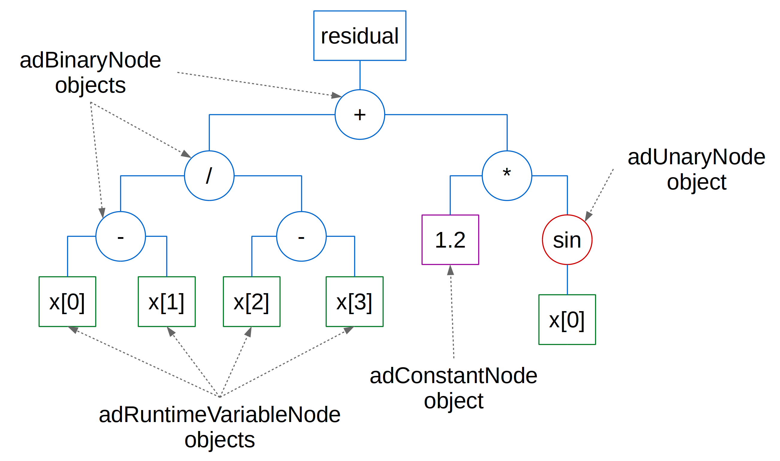
Fig. 6.2 Evaluation Tree

As it has been described in the previous sections, domains, parameters, and variables contain functions that return adouble/adouble_array objects used to construct the evaluation trees. These functions include functions to get a value of a parameter/variable (__call__()), a time or a partial derivative of a variable (functions dt(), d(), or d2()) or functions to obtain an array of values, time or partial derivatives (array(), dt_array(), d_array(), and d2_array()).

6.2.7.6. Defining boundary conditions

DAE tools in general support all types of boundary conditions such as the Dirichlet, Neumann and Robin. As an example, a simple heat transfer model is considered: heat conduction through a very thin rectangular plate. At one side (at y = 0) the Dirichlet boundary conditions are prescribed (the constant temperature: 500 K) while at the opposite end the Neumann boundary conditions (the constant flux: \(10^6 {W}/{m^2}\)). The model is described by a single distributed equation:

\[\rho c_p {{dT(x,y)} \over {dt}} - k \left( {\partial^2 T(x,y) \over \partial x^2} + {\partial^2 T(x,y) \over \partial y^2} \right) = 0; \forall x \in [0, nx], \forall y \in (0, ny)\]

specified as:

# Notation:
#  - T is a variable distributed on x and y domains
#  - rho, k, and cp are parameters
eq = model.CreateEquation("MyEquation")
dx = eq.DistributeOnDomain(x, eClosedClosed)
dy = eq.DistributeOnDomain(y, eOpenOpen)
eq.Residual = rho() * cp() * dt(T(dx,dy)) - k() * ( d2(T(dx,dy), x) + d2(T(dx,dy), y) )

The equation is distributed on the y domain open on both ends; thus, the additional equations (boundary conditions at y = 0 and y = ny-1 points) need to be specified to make the system well posed:

\[\begin{split}T(x,y) &= 500; \forall x \in [0, nx], y = 0 \\ -k {\partial T(x,y) \over \partial y} &= 10^6; \forall x \in [0, nx], y = ny\end{split}\]

which is in DAE Tools given as:

# The Dirichlet boundary conditions at the "bottom edge" :
bceq = model.CreateEquation("Bottom_BC")
dx = bceq.DistributeOnDomain(x, eClosedClosed)
dy = bceq.DistributeOnDomain(y, eLowerBound)
bceq.Residual = T(dx,dy) - Constant(500 * K)  # Constant temperature (500 K)

# The Neumann boundary conditions at the "top edge":
bceq = model.CreateEquation("Top_BC")
dx = bceq.DistributeOnDomain(x, eClosedClosed)
dy = bceq.DistributeOnDomain(y, eUpperBound)
bceq.Residual = - k() * d(T(dx,dy), y) - Constant(1E6 * W/m**2)  # Constant flux (1E6 W/m2)

6.2.7.7. Making equations more readable

Equations residuals can be made more readable by defining some auxiliary functions (as illustrated in Tutorial 2):

def DeclareEquations(self):
    daeModel.DeclareEquations(self)

    # Auxiliary functions and objects
    rho     = self.rho()
    Q       = lambda i:      self.Q(i)
    cp      = lambda x,y:    self.cp(x,y)
    k       = lambda x,y:    self.k(x,y)
    T       = lambda x,y:    self.T(x,y)
    dT_dt   = lambda x,y: dt(self.T(x,y))
    dT_dx   = lambda x,y:  d(self.T(x,y), self.x, eCFDM)
    dT_dy   = lambda x,y:  d(self.T(x,y), self.y, eCFDM)
    d2T_dx2 = lambda x,y: d2(self.T(x,y), self.x, eCFDM)
    d2T_dy2 = lambda x,y: d2(self.T(x,y), self.y, eCFDM)

    eq = self.CreateEquation("HeatBalance", "Heat balance equation valid on the open x and y domains")
    x = eq.DistributeOnDomain(self.x, eOpenOpen)
    y = eq.DistributeOnDomain(self.y, eOpenOpen)
    eq.Residual = rho * cp(x,y) * dT_dt(x,y) - k(x,y) * (d2T_dx2(x,y) + d2T_dy2(x,y))

    eq = self.CreateEquation("BC_bottom", "Neumann boundary conditions at the bottom edge (constant flux)")
    x = eq.DistributeOnDomain(self.x, eOpenOpen)
    y = eq.DistributeOnDomain(self.y, eLowerBound)
    eq.Residual = -k(x,y) * dT_dy(x,y) - Q(0)

    eq = self.CreateEquation("BC_top", "Neumann boundary conditions at the top edge (constant flux)")
    x = eq.DistributeOnDomain(self.x, eOpenOpen)
    y = eq.DistributeOnDomain(self.y, eUpperBound)
    eq.Residual = -k(x,y) * dT_dy(x,y) - Q(1)

    eq = self.CreateEquation("BC_left", "Neumann boundary conditions at the left edge (insulated)")
    x = eq.DistributeOnDomain(self.x, eLowerBound)
    y = eq.DistributeOnDomain(self.y, eClosedClosed)
    eq.Residual = dT_dx(x,y)

    eq = self.CreateEquation("BC_right", " Neumann boundary conditions at the right edge (insulated)")
    x = eq.DistributeOnDomain(self.x, eUpperBound)
    y = eq.DistributeOnDomain(self.y, eClosedClosed)
    eq.Residual = dT_dx(x,y)

Obviously, the heat conduction equation from Tutorial 2:

...

eq.Residual = rho * cp(x,y) * dT_dt(x,y) - k(x,y) * (d2T_dx2(x,y) + d2T_dy2(x,y))

is much more readable than the same equation from Tutorial 1:

...

eq.Residual = self.rho() * self.cp() * dt(self.T(x,y)) - \
              self.k() * (d2(self.T(x,y), self.x, eCFDM) + d2(self.T(x,y), self.y, eCFDM))

6.2.8. State Transition Networks

Discontinuous equations are equations that take different forms subject to certain conditions. In DAE Tools they are modelled using the concept of State Transition Networks (STN). State Transition Networks can be:

1. Reversible (internally described by daeIF class)

2. Irreversible (internally described by daeSTN class)

Every STN consists of two or more states (daeState class). Each state is described by a set of equations and conditions for transitions between states. Irreversible STNs can optionally contain a set of actions to be performed when a specified logical condition is satisfied. At any given moment, there is one active state.

For example, a flow of fluid through a pipe is described by three different regimes:

• Laminar: if Reynolds number is less than 2,100

• Transient: if Reynolds number is greater than 2,100 and less than 10,000

• Turbulent: if Reynolds number is greater than 10,000

From any of these three states the system can go to any other state. This type of discontinuities is called a reversible discontinuity and constructed using the IF(), ELSE_IF(), ELSE() and END_IF() functions:

IF(Re() <= 2100)                    # Laminar flow
#... (equations go here)

ELSE_IF(Re() > 2100 & Re() < 10000) # Transient flow
#... (equations go here)

ELSE()                              # Turbulent flow
#... (equations go here)

END_IF()

The comparison operators operate on adouble objects and floating point values. Units consistency is strictly checked and expressions including plain numbers values are allowed only if a variable or parameter is dimensionless. The following expressions are valid:

# Notation:
#  - T is a variable with units: K
#  - m is a variable with units: kg
#  - p is a dimensionless parameter

# T < 0.5 K
T() < Constant(0.5 * K)

# (T >= 300 K) or (m < 1 kg)
(T() >= Constant(300 * K)) | (m < Constant(0.5 * kg))

# p <= 25.3 (use of the Constant function not necessary)
p() <= 25.3

Reversible discontinuities can be symmetrical and non-symmetrical. The above example is symmetrical. Non-symmetrical STNs are used to describe the concept of hysteresis.

Discontinuities can also be irreversible. For instance, a CPU and its power dissipation can operate in three operating modes:

• Normal mode

  • switch to Power saving mode if CPU load is below 5%

  • switch to Fried mode if the temperature is above 110 degrees

• Power saving mode

  • switch to Normal mode if CPU load is above 5%

  • switch to Fried mode if the temperature is above 110 degrees

• Fried mode

  • Damn, no escape from here… go to the nearest shop and buy a new one! Or, donate some money to DAE Tools project :-)

From the Normal mode the system can either go to the Power saving mode or to the Fried mode. The same stands for the Power saving mode: the system can either go to the Normal mode or to the Fried mode. However, once the temperature exceeds 110 degrees the CPU dies (let’s say it is heavily overclocked) and the system remains in this state permanently. This type of discontinuities is called an irreversible discontinuity and can be described using STN(), STATE(), END_STN() functions:

STN("CPU")

STATE("Normal")
#... (equations go here)
ON_CONDITION( CPULoad() < 0.05,       switchToStates = [ ("CPU", "PowerSaving") ] )
ON_CONDITION( T() > Constant(110*K),  switchToStates = [ ("CPU", "Fried") ] )

STATE("PowerSaving")
#... (equations go here)
ON_CONDITION( CPULoad() >= 0.05,      switchToStates = [ ("CPU", "Normal") ] )
ON_CONDITION( T() > Constant(110*K),  switchToStates = [ ("CPU", "Fried") ] )

STATE("Fried")
#... (equations go here)

END_STN()

The function ON_CONDITION() is used to define actions to be performed when the specified condition is satisfied. In addition, the function ON_EVENT() can be used to define actions to be performed when an event is triggered on a specified event port. Details on how to use ON_CONDITION() and ON_EVENT() functions can be found in the OnCondition actions and OnEvent actions sections, respectively.

More information about state transition networks can be found in daeSTN, daeIF and in Tutorials.

6.2.9. OnCondition actions

The function ON_CONDITION() is used to define actions to be performed when a specified condition is satisfied. The available actions include:

• Changing the active state in specified State Transition Networks (argument switchToStates)

• Re-assigning or re-initialising specified variables (argument setVariableValues)

• Triggering an event on the specified event ports (argument triggerEvents)

• Executing user-defined actions (argument userDefinedActions)

Nota bene

OnCondition actions can be added to models or to states in State Transition Networks (daeSTN or daeIF):

• When added to a model they remain active throughout the simulation

• When added to a state they become active only when the parent state becomes active

Nota bene

switchToStates, setVariableValues, triggerEvents and userDefinedActions are empty by default. The user has to specify at least one action.

For instance, to execute some actions when the temperature becomes greater than 340 K the following can be used:

def DeclareEquations(self):
    ...

    self.ON_CONDITION( T() > Constant(340*K), switchToStates     = [ ('STN', 'StateName'), ... ],
                                              setVariableValues  = [ (variable, newValue), ... ],
                                              triggerEvents      = [ (eventPort, eventMessage), ... ],
                                              userDefinedActions = [ userDefinedAction, ... ] )

where the first argument of the ON_CONDITION() function is a condition specifying when the actions will be executed and:

• switchToStates is a list of tuples (string ‘STN Name’, string ‘State name to activate’)

• setVariableValues is a list of tuples (daeVariable object, adouble object)

• triggerEvents is a list of tuples (daeEventPort object, adouble object)

• userDefinedActions is a list of user defined objects derived from the base daeAction class

More details on how to use ON_CONDITION() function can be found in Tutorial 13.

6.2.10. OnEvent actions

The function ON_EVENT() is used to define actions to be performed when an event is triggered on the specified event port. The same type of actions are available as in the ON_CONDITION() function.

Nota bene

OnEvent actions can be added to models or to states in State Transition Networks (daeSTN or daeIF):

• When added to a model they remain active throughout the simulation

• When added to a state they become active only when the parent state becomes active

Nota bene

switchToStates, setVariableValues, triggerEvents and userDefinedActions are empty by default. The user has to specify at least one action.

For instance, to execute some actions when an event is triggered on an event port the following can be used:

def DeclareEquations(self):
    ...

    self.ON_EVENT( eventPort, switchToStates     = [ ('STN', 'StateName'), ... ],
                              setVariableValues  = [ (variable, newValue), ... ],
                              triggerEvents      = [ (eventPort, eventMessage), ... ],
                              userDefinedActions = [ userDefinedAction, ... ] )

where the first argument of the ON_EVENT() function is the daeEventPort object to be monitored for events, while the rest of the arguments is the same as in the ON_CONDITION() function.

More details on how to use ON_EVENT() function can be found in Tutorial 13.

6.2.11. User-defined actions

User-defined actions are executed in a response to a specified condition in OnCondition handlers or in a response to an event triggered in OnEvent handlers.

They are created by deriving a class from the daeAction base and implementing the Execute() function. The Execute() function takes no arguments. If some information from the model is required they should be specified in the constructor.

User-defined actions do not return a value and should not change the values of variables (other types of actions must be used for that purpose), but perform some user-defined operations. The source code for a simple action that prints a message with the data sent to a specified event port is given below:

# User-defined action executed when an event is triggered on a specified event port.
class simpleUserAction(daeAction):
    def __init__(self, eventPort):
        daeAction.__init__(self)

        # Store the daeEventPort object for later use.
        self.eventPort = eventPort

    def Execute(self):
        # The floating point value of the data sent when the event is triggered
        # can be retrieved using the daeEventPort.EventData property.
        msg = 'simpleUserAction executed; input data = %f' % self.eventPort.EventData

        print('********************************************************')
        print(msg)
        print('********************************************************')

Notate bene

User-defined action objects should be instantiated in the DeclareEquations() function if they access parameters’ and variables’ symbolic representations (available only there).

User-defined action objects must be stored in the model, otherwise they will get destroyed when they go out of scope.

def DeclareEquations(self):
    ...

    # User-defined action objects should be stored in the model, otherwise
    # they will get destroyed when they go out of scope.
    self.action = simpleUserAction(self.eventPort)

    # The actions executed when the event on the inlet 'eventPort' event port is received.
    # daeEventPort defines the operator() which returns adouble object that can be used
    # at the moment when the action is executed to get the value of the event data.
    self.ON_EVENT(self.eventPort, userDefinedActions = [self.action])

More details on how to use user-defined actions can be found in Tutorial 13.

6.2.12. External functions

The concept of external functions in DAE Tools is used to handle and evaluate user-defined functions or functions from external libraries. External functions can return scalar (daeScalarExternalFunction) or vector (daeVectorExternalFunction) values.

Nota bene

The vector external functions are not implemented at the moment.

External functions are created by deriving a class from the daeScalarExternalFunction base, specifying its arguments in the constructor and implementing the Calculate() function. The source code for a simple \(F(x) = x ^ 2\) external function is given below:

class F(daeScalarExternalFunction):
    def __init__(self, Name, parentModel, units, x):
        # Instantiate the scalar external function by specifying
        # the dictionary with arguments {'name' : adouble-object}
        arguments = {}
        arguments["x"]  = x

        daeScalarExternalFunction.__init__(self, Name, parentModel, units, arguments)

    def Calculate(self, values):
        # Calculate function is used to calculate a value and a derivative of the external
        # function per given argument (if requested). Here, a simple function is given by:
        #    F(x) = x**2

        # Procedure:
        # 1. Get the arguments from the dictionary 'values': {'arg-name' : adouble-object}.
        #    Every adouble object has two properties: Value and Derivative that can be
        #    used to evaluate function or its partial derivatives per arguments
        #    (partial derivatives are used to fill in a Jacobian matrix necessary to solve
        #    a system of non-linear equations using the Newton method).
        x = values["x"]

        # 2. Always calculate the value of a function (the derivative is zero by default).
        res = adouble(x.Value ** 2)

        # 3. If a function derivative per one of its arguments is requested,
        #    the derivative part of that argument will be non-zero.
        #    In that case, investigate which derivative is requested and calculate it
        #    using the chain rule: f'(x) = x' * df(x)/dx
        if x.Derivative != 0:
            # A derivative per 'x' was requested; its value is: x' * 2x
            res.Derivative = x.Derivative * (2 * x.Value)

        # 4. Return the result as a adouble object (contains both a value and a derivative)
        return res

Notate bene

External function objects must be instantiated in the DeclareEquations() function since they access parameters’ and variables’ symbolic representations (available only there).

External function objects must be stored in the model, otherwise they will get destroyed when they go out of scope.

def DeclareEquations(self):
    ...

    # Create external function (it has to be created in DeclareEquations!),
    # specify its units (here for simplicity dimensionless) and
    # arguments (here only a single argument: x)
    # External function objects should be stored in the model, otherwise
    # they will get destroyed when they go out of scope.
    self.F = F("F", self, unit(), self.x())

    # External function can now be used in daetools equations.
    # Its value can be obtained using the operator() (python special function __call__)
    eq = self.CreateEquation("...", "...")
    eq.Residual = ... self.F() ...

A more complex example is given in the Tutorial 14. There, the external function concept is used to interpolate a set of values using the scipy.interpolate.interp1d object.

class extfn_interp1d(daeScalarExternalFunction):
    def __init__(self, Name, parentModel, units, times, values, Time):
        arguments = {}
        arguments["t"] = Time

        # Instantiate interp1d object and initialise interpolation using supplied (time,y) values.
        self.interp = scipy.interpolate.interp1d(times, values)

        # During the solver iterations, the function is called very often with the same arguments.
        # Therefore, cache the last interpolated value to speed up a simulation.
        self.cache = None

        daeScalarExternalFunction.__init__(self, Name, parentModel, units, arguments)

    def Calculate(self, values):
        # Get the argument from the dictionary of arguments' values.
        time = values["t"].Value

        # Here we do not need to return a derivative for it is not a function of variables.

        # First check if an interpolated value was already calculated during the previous call.
        # If it was, return the cached value (the derivative part is always equal to zero in this case).
        if self.cache:
            if self.cache[0] == time:
                return adouble(self.cache[1])

        # The time received is not in the cache and has to be interpolated.
        # Convert the result to float datatype since daetools can't accept
        # numpy.float64 types as arguments at the moment.
        interp_value = float(self.interp(time))
        res = adouble(interp_value, 0)

        # Save it in the cache for later use.
        self.cache = (time, res.Value)

        return res

The extfn_interp1d class is used here to approximate some function f:

\[y = f(t) = 2t\]

using its t ad y values:

def DeclareEquations(self):
    ...

    # Create scipy.interp1d interpolation external function.
    # Create 'times' and 'values' arrays to be used for interpolation:
    times  = numpy.arange(0.0, 1000.0)
    values = 2*times
    # The external function accepts only a single argument: the current time in the simulation
    # that can be obtained using the Time() daetools function.
    # The external function units are seconds.
    self.interp1d = extfn_interp1d("interp1d", self, s, times, values, Time())

Alternatively, DAE Tools can utilise functions defined in shared libraries via daeCTypesExternalFunction class. As an argument it accepts a function pointer from libraries loaded using Python ctypes. Sample usage can be found in the Tutorial 14:

def DeclareEquations(self):
    ...

    # Load the library:
    self.ext_lib = ctypes.CDLL("libheat_function.so")

    # Function arguments:
    arguments = {}
    arguments['m']     = self.m()
    arguments['cp']    = self.cp()
    arguments['dT/dt'] = dt(self.T())

    # Function pointer ('calculate' function is used):
    function_ptr = self.ext_lib.calculate

    self.exfnHeat2 = daeCTypesExternalFunction("heat_function", self, W, function_ptr, arguments)

The calculate function is defined in the heat_function c shared library:

#include <string.h>

typedef struct
{
    double Value;
    double Derivative;
}
adouble_c;

#if defined(_WIN32) || defined(WIN32) || defined(WIN64) || defined(_WIN64)
#define DLLEXPORT  extern "C" __declspec(dllexport)
#else
#define DLLEXPORT
#endif

DLLEXPORT adouble_c calculate(const adouble_c values[], const char* names[], int no_arguments);

adouble_c calculate(const adouble_c values[], const char* names[], int no_arguments)
{
    adouble_c result;
    memset(&result, 0, sizeof(adouble_c));

    /* Get the arguments' values. */
    adouble_c m, cp, dT_dt;
    for(int i = 0; i < no_arguments; i++)
    {
        if(strcmp(names[i], "m") == 0)
            m = values[i];
        else if(strcmp(names[i], "cp") == 0)
            cp = values[i];
        else if(strcmp(names[i], "dT/dt") == 0)
            dT_dt = values[i];
    }

    /* Calculate the value. */
    result.Value = m.Value * cp.Value * dT_dt.Value;

    /* Calculate the derivative. */
    if(m.Derivative != 0) /* A derivative per 'm' was requested */
        result.Derivative = m.Derivative * (cp.Value * dT_dt.Value);
    else if(cp.Derivative != 0) /* A derivative per 'cp' was requested */
        result.Derivative = cp.Derivative * (m.Value * dT_dt.Value);
    else if(dT_dt.Derivative != 0) /* A derivative per 'dT_dt' was requested */
        result.Derivative = dT_dt.Derivative * (m.Value * cp.Value);

    return result;
}

The library can be compiled using the following commands:

# GNU/Linux gcc:
gcc -fPIC -shared -o libheat_function.so tutorial4_heat_function.c

# macOS gcc:
gcc -fPIC -dynamiclib -o libheat_function.dylib tutorial14_heat_function.c

# Windows vc++:
cl /LD tutorial14_heat_function.c /link /dll /out:heat_function.dll

6.3. Numerical Methods for Partial Differential Equations

6.3.1. The Finite Difference Method

DAE Tools support numerical simulation of partial differential equations on structured grids using the Finite Difference Method. Three different methods are provided:

• Backward Finite Difference method (eBFDM)

• Forward Finite Difference method (eFFDM)

• Center Finite Difference method (eCFDM)

The partial derivatives of the first and second order can be specified using the functions d() and d2().

As an illustration, the 1D convection-diffusion-reaction equation:

\[\begin{split}{\partial c \over \partial t} + u {\partial c \over \partial x} - D {\partial^2 c \over \partial x^2} &= s(x), \forall x \in \left( 0,L \right] \\ c(0) &= 0.0\end{split}\]

can be specified using the Center Finite Difference Method:

class modTutorial(daeModel):
    ...
    def DeclareEquations(self):
        daeModel.DeclareEquations(self)

        # Notation:
        #  - c is a state variable
        #  - x is a domain object
        #  - u is velocity

        # Declare some auxiliary functions to make equations more readable
        c       = lambda i: self.c(i)
        dc_dt   = lambda x: dt(c(x))
        dc_dx   = lambda x: d (c(x), self.x, eCFDM)
        d2c_dx2 = lambda x: d2(c(x), self.x, eCFDM)
        s       = lambda i: c(i)**2

        # Declare the Convection-Diffusion-Reaction equation distributed on (0, L]:
        eq = self.CreateEquation("c")
        eq.DistributeOnDomain(self.x, eOpenClosed)
        eq.Residual = dc_dt(x) + u * dc_dx(x) - D * d2c_dx2(x) - s(x)

        # Boundary conditions at x = 0:
        eq = self.CreateEquation("c(0)")
        eq.Residual = c(0) - 0.0

6.3.2. The Finite Volume Method

DAE Tools support numerical simulation of partial differential equations on 1D structured grids using the Finite Volume Method (high-resolution upwind scheme with flux limiter).

Consider the 1D convection-diffusion-reaction equation:

\[{\partial c \over \partial t} + u {\partial c \over \partial x} - D {\partial^2 c \over \partial x^2} = s(x)\]

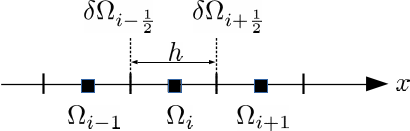
A cell-centered finite-volume discretisation yields the semi-discrete equation [1] [2]:

\[\int_{\Omega_i} {\partial c_i \over \partial t} dx + u \left[ c_{i + {1 \over 2}} - c_{i - {1 \over 2}} \right] - D \left[ \left( \partial c \over \partial x \right)_{i + {1 \over 2}} - \left( \partial c \over \partial x \right)_{i - {1 \over 2}} \right] = \int_{\Omega_i} s_i dx\]

where the half-integer indices refer to cell faces \(\delta\Omega_{i-{1 \over 2}}\) and \(\delta\Omega_{i+{1 \over 2}}\) between cell centers \(\Omega_{i-1}\) and \(\Omega_i\) as presented in the figure below:

The accuracy of the above finite volume discretisation is determined by the way in which the cell-face fluxes are computed. Applying the high-resolution upwind scheme with flux limiter [1] [2] for the cell-face state \(c_{i+{1 \over 2}}\) results in the following equation:

\[{c}_{i + {1 \over 2}} = c_i + \phi \left( r_{i + {1 \over 2}} \right) \left( c_i - c_{i-1} \right)\]

where \(\phi\) is the flux limiter function and \(r_{i + {1 \over 2}}\) the upwind ratio of consecutive solution gradients:

\[r_{i + {1 \over 2}} = {{c_{i+1} - c_{i} + \epsilon} \over {c_{i} - c_{i-1} + \epsilon}}\]

There is a large number of flux limiters [3] implemented in DAE Tools:

• CHARM [not 2nd order TVD] (Zhou, 1995):

  \(\phi(r)= \begin{cases} \frac{r\left(3r+1\right)}{\left(r+1\right)^{2}} & r>0, \lim_{r \rightarrow \infty} \phi(r)=3 \\ 0 & otherwise \end{cases}\)

• HCUS (not 2nd order TVD) (Waterson and Deconinck, 1995):

  \(\phi(r) = \frac{ 1.5 \left(r+\left| r \right| \right)}{ \left(r+2 \right)} , \lim_{r \rightarrow \infty}\phi_{hc}(r) = 3\)

• HQUICK (not 2nd order TVD) (Waterson and Deconinck, 1995):

  \(\phi(r) = \frac{2 \left(r + \left|r \right| \right)}{ \left(r+3 \right)}, \lim_{r \rightarrow \infty}\phi_{hq}(r) = 4\)

• Koren (Koren, 1993):

  \(\phi(r) = \max \left[ 0, \min \left(2 r, \left(2 + r \right)/3, 2 \right) \right], \lim_{r \rightarrow \infty}\phi(r) = 2\)

• minmod - symmetric (Philip and Roe, 1986):

  \(\phi (r) = \max \left[ 0 , \min \left( 1 , r \right) \right], \lim_{r \rightarrow \infty}\phi(r) = 1\)

• monotonized central (MC) – symmetric (van Leer, 1977):

  \(\phi (r) = \max \left[ 0 , \min \left( 2 r, 0.5 (1+r), 2 \right) \right] , \lim_{r \rightarrow \infty}\phi(r) = 2\)

• Osher (Chatkravathy and Osher, 1983):

  \(\phi (r) = \max \left[ 0 , \min \left( r, \beta \right) \right], \left(1 \leq \beta \leq 2 \right), \lim_{r \rightarrow \infty}\phi (r) = \beta\)

• ospre - symmetric (Waterson and Deconinck, 1995):

  \(\phi (r) = \frac{1.5 \left(r^2 + r \right) }{\left(r^2 + r +1 \right)} , \lim_{r \rightarrow \infty}\phi (r) = 1.5\)

• smart (not 2nd order TVD) (Gaskell and Lau, 1988):

  \(\phi(r) = \max \left[ 0, \min \left(2 r, \left(0.25 + 0.75 r \right), 4 \right) \right], \lim_{r \rightarrow \infty}\phi(r) = 4\)

• superbee – symmetric (Roe, 1986):

  \(\phi (r) = \max \left[ 0, \min \left( 2 r , 1 \right), \min \left( r, 2 \right) \right] , \lim_{r \rightarrow \infty}\phi (r) = 2\)

• Sweby – symmetric (Sweby, 1984):

  \(\phi (r) = \max \left[ 0 , \min \left( \beta r, 1 \right), \min \left( r, \beta \right) \right], \left(1 \leq \beta \leq 2 \right), \lim_{r \rightarrow \infty}\phi (r) = \beta\)

• UMIST (Lien and Leschziner, 1994):

  \(\phi(r) = \max \left[ 0, \min \left(2 r, \left(0.25 + 0.75 r \right), \left(0.75 + 0.25 r \right), 2 \right) \right] , \lim_{r \rightarrow \infty}\phi(r) = 2\)

• van Albada 1 - symmetric (van Albada, et al., 1982):

  \(\phi (r) = \frac{r^2 + r}{r^2 + 1 } , \lim_{r \rightarrow \infty}\phi (r) = 1\)

• van Albada 2 : alternative form (not 2nd order TVD; Kermani, 2003)

  \(\phi (r) = \frac{2 r}{r^2 + 1}, \lim_{r \rightarrow \infty}\phi(r) = 0\)

• van Leer - symmetric (van Leer, 1974):

  \(\phi (r) = \frac{r + \left| r \right| }{1 + \left| r \right| } , \lim_{r \rightarrow \infty}\phi (r) = 2\)

For the diffusive flux, the gradient \(\left( \partial c \over \partial x \right)_{i + {1 \over 2}}\) is evaluated using the standard second-order accurate central difference formula:

\[\left( \partial c \over \partial x \right)_{i + {1 \over 2}} = {{c_{i+1} - c_i} \over h}\]

except at the inflow and outflow boundaries where:

\[\begin{split}\left( \partial c \over \partial x \right)_{{1 \over 2}} &= {{-8c_{1 \over 2} + 9c_1 - c_2} \over 3h} \\ \left( \partial c \over \partial x \right)_{n + {1 \over 2}} &= {{8c_{n + {1 \over 2}} - 9c_n + c_{n-1}} \over 3h}\end{split}\]

The above convection-diffusion-reaction equation can be specified using the daeHRUpwindSchemeEquation class with the following functions:

• Accumulation term in the cell-centered finite-volume discretisation: dc_dt():

  \(dc\_dt(i) = \int_{\Omega_i} {\partial c_i \over \partial t} dx\)

• Convection term in the cell-centered finite-volume discretisation: dc_dx() (may contain the \(\mathbf{S} = {1 \over u} \int_{\Omega_i} s(x) dx\) integral for the consistent discretisation of the convection and the source terms):

  \(dc\_dx(i) = c_{i + {1 \over 2}} - c_{i - {1 \over 2}}\)

  or (if the source integral \(\mathbf{S}\) has been specified):

  \(dc\_dx(i) = \left( c_{i + {1 \over 2}} - \mathbf{S}_{i + {1 \over 2}} \right) - \left( c_{i - {1 \over 2}} - \mathbf{S}_{i - {1 \over 2}} \right)\)

• Diffusion term in the cell-centered finite-volume discretisation: d2c_dx2():

  \(d2c\_dx2(i) = \left( \partial c \over \partial x \right)_{i + {1 \over 2}} - \left( \partial c \over \partial x \right)_{i - {1 \over 2}}\)

• Source term in the cell-centered finite-volume discretisation: source():

  \(source(i) = \int_{\Omega_i} s_i dx\)

as given in the example below:

class modTutorial(daeModel):
    def __init__(self, Name, Parent = None, Description = ""):
        daeModel.__init__(self, Name, Parent, Description)

    def DeclareEquations(self):
        daeModel.DeclareEquations(self)

        xp = self.x.Points
        Nx = self.x.NumberOfPoints

        c = lambda i: self.c(i)

        # 1. Declare the HR upwind scheme object:
        #     - c is a state variable
        #     - x is a domain object
        #     - Phi_Koren is a flux limiter function
        hr = daeHRUpwindSchemeEquation(self.c, self.x, daeHRUpwindSchemeEquation.Phi_Koren, 1e-10)

        # 2. Define the source term function
        def s(i):
            return self.c(i)**2

        # 3. Declare the Convection-Diffusion-Reaction equation distributed on (0, L]:
        for i in range(1, Nx):
            eq = self.CreateEquation("c(%d)" % i)
            eq.Residual = hr.dc_dt(i) + u * hr.dc_dx(i) - D * hr.d2c_dx2(i) - hr.source(s,i)

        # Boundary conditions at x=0:
        eq = self.CreateEquation("c(0)")
        eq.Residual = c(0) - ...

It is desired that the discretisation of the source term is consistent with that of the advection operator. For this purpose, if the source term integral: \(S(x) = {1 \over u} \int_{\Omega_i} s(x) dx\) can be calculated analytically, the convection term can be rewritten as:

\[{\partial c \over \partial t} + u {\partial (c-\mathbf{S}) \over \partial x} - D {\partial^2 c \over \partial x^2} = 0\]

and the semi-discrete equation becomes:

\[\int_{\Omega_i} {\partial c_i \over \partial t} dx + u \left[ \left( c_{i + {1 \over 2}} - \mathbf{S}_{i + {1 \over 2}} \right) - \left( c_{i - {1 \over 2}} - \mathbf{S}_{i - {1 \over 2}} \right) \right] - D \left[ \left( \partial c_i \over \partial x \right)_{i + {1 \over 2}} - \left( \partial c_i \over \partial x \right)_{i - {1 \over 2}} \right] = 0\]

The example above now becomes:

class modTutorial(daeModel):
    def __init__(self, Name, Parent = None, Description = ""):
        daeModel.__init__(self, Name, Parent, Description)

    def DeclareEquations(self):
        daeModel.DeclareEquations(self)

        xp = self.x.Points
        Nx = self.x.NumberOfPoints

        c = lambda i: self.c(i)

        # 1. Declare the HR upwind scheme object:
        #     - c is a state variable
        #     - x is a domain object
        #     - u is velocity
        #     - Phi_Koren is a flux limiter function
        hr = daeHRUpwindSchemeEquation(self.c, self.x, daeHRUpwindSchemeEquation.Phi_Koren, 1e-10)

        # 2. Consistent discretisation of convection and source terms:
        #    Calculate an analytical integral of the source term S = 1/u * Integral(s(x)*dx)
        def S(i):
            C1 = 0.0
            return c(i)**2 / 3 + C1

        # 3. Declare the Convection-Diffusion-Reaction equation distributed on (0, L]
        #    (with the S integral in the convection term):
        for i in range(1, Nx):
            eq = self.CreateEquation("c(%d)" % i)
            eq.Residual = hr.dc_dt(i) + u * hr.dc_dx(i, S) - D * hr.d2c_dx2(i)

        # Boundary Conditions:
        eq = self.CreateEquation("c(0)")
        eq.Residual = c(0) - ...

Footnotes

[1] (1,2)

B. Koren. A robust upwind discretisation method for advection, diffusion and source terms. In: Vreugdenhil CB, Koren B, editors. Numerical Methods for Advection–Diffusion Problems. Braunschweig: Vieweg; 1993. ISBN-10:3528076453.

[2] (1,2)

B. Koren. A robust upwind discretization method for advection, diffusion and source terms. Department of Numerical Mathematics. Report NM-R9308 (1993). PDF

[3]

Flux-limiter functions on Wikipedia

6.3.3. The Finite Element Method

DAE Tools support numerical simulation of partial differential equations on unstructured grids using the Finite Element method. The main idea is to utilise available state-of-the-art Finite Element libraries (i.e. deal.II) for low-level tasks such as mesh loading, management of finite element spaces, degrees of freedom, assembly of the system stiffness and mass matrices and the system load vector, setting the boundary conditions etc.. After the assembly phase in an external library the matrices are used to generate a set of equations in the following form:

\[\left[ M_{ij} \right] \left\{ {dx_j} \over {dt} \right\} + \left[ A_{ij} \right] \left\{ x_j \right\} = \left\{ F_i \right\}\]

where \(x_j\) is a state variable, \(M_{ij}\) and \(A_{ij}\) are mass and stiffness matrices and \(F_i\) is the load vector. This system is in a general case a DAE system, although it can also be a linear or a non-linear (if the mass matrix is zero). The generated set of equations are solved together with the rest of equations in the model.

The unique feature of this approach is a capability to use DAE Tools objects (parameters and variables) as a native data type in deal.II functions to specify boundary conditions, time varying coefficients and source terms. This way, the non-linear finite element systems are automatically supported and the equations resulting from the finite element discretisation are fully integrated with the rest of the model equations. Moreover, multiple FE systems can be created and coupled together.

The information required (from the modeller’s perspective):

• Mesh file with the specified boundary indicators (integers)

• Variables (degrees of freedom in deal.II) and their Finite Element spaces

• Quadrature formulas for elements and their faces

• The weak form of the problem which contains expressions for the cells’ and boundary faces’ contributions to the system mass and stiffness matrix and the load vector.

The weak form expressions are specified using the DAE Tools API that wraps deal.II concepts used to assembly the matrices/vectors. The weak forms in daetools contain expressions as they would appear in typical nested for loops. In deal.II a typical cell assembly loop (in C++) would look like (i.e. a very simple example given in step-7):

FEValues<dim>             fe_values(...);
std::vector<unsigned int> local_dof_indices;

typename DoFHandler<dim>::active_cell_iterator cell = dof_handler.begin_active(),
                                               endc = dof_handler.end();
for(; cell != endc; ++cell)
{
    fe_values.reinit(cell);
    cell->get_dof_indices(local_dof_indices);

    for(unsigned int q_point = 0; q_point < n_q_points; ++q_point)
    {
        for(unsigned int i = 0; i < dofs_per_cell; ++i)
        {
            for(unsigned int j = 0; j < dofs_per_cell; ++j)
            {
                cell_matrix(i,j) += ((fe_values.shape_grad(i,q_point) *
                                      fe_values.shape_grad(j,q_point)
                                      +
                                      fe_values.shape_value(i,q_point) *
                                      fe_values.shape_value(j,q_point)) *
                                    fe_values.JxW(q_point));
            }

            cell_rhs(i) += (fe_values.shape_value(i,q_point) *
                            rhs_values [q_point] * fe_values.JxW(q_point));
        }
    }
}

An equivalent problem in DAE Tools creates an execution context used in a generic loop to evaluate the cell/face contributions:

FEValues<dim>             fe_values(...);
std::vector<unsigned int> local_dof_indices;

// Create evaluation context objects where the expressions will be evaluated:
feCellContext<dim> cellContext(fe_values, local_dof_indices, ...);

typename DoFHandler<dim>::active_cell_iterator cell = dof_handler.begin_active(),
                                               endc = dof_handler.end();
for(; cell != endc; ++cell)
{
    // Update the evaluation context with the current cell.
    // It will call fe_values.reinit(cell), cell->get_dof_indices(local_dof_indices) etc.
    update(cellContext, cell);

    for(unsigned int q_point = 0; q_point < n_q_points; ++q_point)
    {
        // update cellContext with the current quadrature point index

        for(unsigned int i = 0; i < dofs_per_cell; ++i)
        {
            // update cellContext with the current i loop dof index

            for(unsigned int j = 0; j < dofs_per_cell; ++j)
            {
                // update cellContext with the current j loop dof index

                cell_matrix(i,j) += evaluate(cell_contribution_to_stiffness_matrix, cellContext);
            }

            // update cellContext with the current i, j, q indices

            cell_rhs(i) += evaluate(cell_contribution_to_load_vector, cellContext);
        }
    }
}

Apart from specifying the weak formulation using the single expressions evaluated in a generic loop as shown above, tuples of expressions representing independent terms evaluated in the q, i and j loops can be also used. This is useful for complex weak form expressions involving non-linear terms (i.e. dof approximations) and results in simpler expressions and a faster evaluation. The usage of separate items for different loop iterations is illustrated below:

FEValues<dim>             fe_values(...);
std::vector<unsigned int> local_dof_indices;

// Create evaluation context objects where the expressions will be evaluated:
feCellContext<dim> cellContext(fe_values, local_dof_indices, ...);

typename DoFHandler<dim>::active_cell_iterator cell = dof_handler.begin_active(),
                                               endc = dof_handler.end();
for(; cell != endc; ++cell)
{
    // Update the evaluation context with the current cell.
    // It will call fe_values.reinit(cell), cell->get_dof_indices(local_dof_indices) etc.
    update(cellContext, cell);

    for(unsigned int q_point = 0; q_point < n_q_points; ++q_point)
    {
        // Temporary storage
        Vector<adouble>     cell_rhs_temp(dofs_per_cell);
        FullMatrix<adouble> cell_matrix_temp(dofs_per_cell, dofs_per_cell);

        // update cellContext with the current quadrature point index

        q_loop_term = evaluate(q_loop_expression, cellContext);

        for(unsigned int i = 0; i < dofs_per_cell; ++i)
        {
            // update cellContext with the current i loop dof index

            i_loop_term = evaluate(i_loop_expression, cellContext);

            for(unsigned int j = 0; j < dofs_per_cell; ++j)
            {
                // update cellContext with the current j loop dof index

                j_loop_term = evaluate(j_loop_expression, cellContext);

                cell_matrix_temp(i,j) += i_loop_term * j_loop_term;
            }

            cell_rhs_temp(i) += i_loop_term;
        }

        cell_rhs_temp    *= q_loop_term;
        cell_matrix_temp *= q_loop_term;
    }

    // Add the temporary data to the cell matrix/vector
    cell_rhs    += cell_rhs_temp;
    cell_matrix += cell_matrix_temp;
}

Obviously, the generic loops can be used to solve many FE problems but not all. However, they can support a large number of problems at the moment. In the future they will be expanded to support a broader class of problems.

Equations produced by the Finite Element matrix assembly can be extremely long/complex. Under the hood, they will be simplified as much as possible. Some examples are given below.

• From Tutorial deal.II 2:

  

• From Tutorial deal.II 3:

  

• From Tutorial deal.II 7:

  

DAE Tools provide four main classes for Finite Element models using deal.II library:

1. dealiiFiniteElementDOF_1D, dealiiFiniteElementDOF_2D and dealiiFiniteElementDOF_3D

   In deal.II it represents a degree of freedom distributed on a finite element domain. In DAE Tools it represents a variable distributed on a finite element domain.

2. dealiiFiniteElementSystem_1D, dealiiFiniteElementSystem_2D and dealiiFiniteElementSystem_3D (implements daeFiniteElementObject)

   It is a wrapper around deal.II FESystem<dim> class and handles all finite element related details. It uses information about the mesh, quadrature and face quadrature formulas, degrees of freedom and the FE weak formulation to assemble the system’s mass matrix (Mij), stiffness matrix (Aij) and the load vector (Fi).

3. dealiiFiniteElementWeakForm_1D, dealiiFiniteElementWeakForm_2D and dealiiFiniteElementWeakForm_3D

   Contains weak form expressions for the contribution of FE cells to the system/stiffness matrices, the load vector, boundary conditions and (optionally) surface/volume integrals (as an output).

4. daeFiniteElementModel

   daeModel-derived class that use system matrices/vectors from the dealiiFiniteElementSystem_nD object to generate a system of equations.

A typical use-case scenario consists of the following steps:

1. The starting point is a definition of the dealiiFiniteElementSystem_nD class (where nD can be 1D, 2D or 3D). That includes specification of:

   • Mesh file in one of the formats supported by deal.II (GridIn)

   • Degrees of freedom (as a python list of dealiiFiniteElementDOF_nD objects). Every dof has a name which will be also used to declare DAE Tools variable with the same name, description, finite element space FE (deal.II FiniteElement<dim> instance) and the multiplicity

   • Quadrature formulas for elements and their faces

2. Creation of daeFiniteElementModel object (similarly to the ordinary DAE Tools model) with the finite element system object as the last argument.

3. Definition of the weak form of the problem using the following functions (a version exist for 1D, 2D and 3D):

   • phi_1D(): corresponds to shape_value in deal.II

   • dphi_1D(): corresponds to shape_grad in deal.II

   • d2phi_1D(): corresponds to shape_hessian in deal.II

   • phi_vector_1D(): corresponds to shape_value of vector dofs in deal.II

   • dphi_vector_1D(): corresponds to shape_grad of vector dofs in deal.II

   • d2phi_vector_1D(): corresponds to shape_hessian of vector dofs in deal.II

   • div_phi_1D(): corresponds to divergence in deal.II

   • JxW_1D(): corresponds to the mapped quadrature weight in deal.II

   • xyz_1D(): returns the point for the specified quadrature point in deal.II

   • normal_1D(): corresponds to the normal_vector in deal.II

   • function_value_1D(): wraps Function<dim> object that returns a value

   • function_gradient_1D(): wraps Function<dim> object that returns a gradient

   • function_adouble_value_1D(): wraps Function<dim,adouble> object that returns adouble value

   • function_adouble_gradient_1D(): wraps Function<dim,adouble> object that returns adouble gradient

   • dof_1D(): returns daetools variable at the given index (adouble object)

   • dof_approximation_1D(): returns FE approximation of a quantity as a daetools variable (adouble object)

   • dof_gradient_approximation_1D(): returns FE gradient approximation of a quantity as a daetools variable (adouble object)

   • dof_hessian_approximation_1D(): returns FE hessian approximation of a quantity as a daetools variable (adouble object)

   • vector_dof_approximation_1D(): returns FE approximation of a vector quantity as a daetools variable (adouble object)

   • vector_dof_gradient_approximation_1D(): returns FE approximation of a vector quantity as a daetools variable (adouble object)

   • adouble_1D(): wraps any daetools expression to be used in matrix assembly

   • tensor1_1D(): wraps deal.II Tensor<rank=1>

   • tensor2_1D(): wraps deal.II Tensor<rank=2>

   • tensor3_1D(): wraps deal.II Tensor<rank=3>

   • adouble_tensor1_1D(): wraps deal.II Tensor<rank=1,adouble>

   • adouble_tensor2_1D(): wraps deal.II Tensor<rank=2,adouble>

   • adouble_tensor3_1D(): wraps deal.II Tensor<rank=3,adouble>

   and constants: fe_i, fe_j and fe_q used to access the current indexes in the DOF and quadrature points loops.

The weak form contains the following contributions:

• Aij - cell contribution to the system stiffness matrix

• Mij - cell contribution to the system mass matrix

• Fi - cell contribution to the system load vector

• boundaryFaceAij - boundary face contribution to the system stiffness matrix

• boundaryFaceFi - boundary face contribution to the load vector

• innerCellFaceAij - inner cell face contribution to the system stiffness matrix

• innerCellFaceFi - inner cell face contribution to the load vector

• functionsDirichletBC - Dirichlet boundary conditions

• surfaceIntegrals - surface integrals

• volumeIntegrals - volume integrals

Example for the Helmholtz problem (step-7 tutorial from deal.II). The strong form of the Helmholtz equation is given by (with Neumann boundary conditions):

\[\begin{split}-\Delta u + u &= f \; in \; \Omega \\ {\mathbf n}\cdot \nabla u &= g \; on \; \delta \Omega\end{split}\]

The weak form of the above equation is:

\[{(\nabla u, \nabla v)}_\Omega + {(u,v)}_\Omega = {(f,v)}_\Omega + {(g,v)}_{\delta \Omega}\]

Cell contributions to the stiffness matrix and the load vector are:

\[\begin{split}A_{ij} &= \left(\nabla \varphi_i, \nabla \varphi_j\right) +\left(\varphi_i, \varphi_j\right) \\ F_i &= \left(f,\varphi_i\right) + \left(g, \varphi_i\right)_{\delta \Omega}\end{split}\]

The c++ implementation in deal.II is given in the step-7 example and in the previous c++ listing. In DAE Tools the above equation is specified in the following way (\(\delta \Omega\) boundary is marked with id = 0 and for simplicity, \(f\) and \(g\) are assumed constant):

class modTutorial(daeModel):
    def __init__(self, Name, Parent = None, Description = ""):
        daeModel.__init__(self, Name, Parent, Description)

        dofs = [dealiiFiniteElementDOF_2D(name='u',
                                          description='u description',
                                          fe = FE_Q_2D(1),
                                          multiplicity=1)]

        self.fe_system = dealiiFiniteElementSystem_2D(meshFilename    = '...',        # path to the .msh file
                                                      quadrature      = QGauss_2D(3), # quadrature formula
                                                      faceQuadrature  = QGauss_1D(3), # face quadrature formula
                                                      dofs            = dofs)         # degrees of freedom

        self.fe_model = daeFiniteElementModel('Helmholtz', self, 'Helholtz problem', self.fe_system)

    def DeclareEquations(self):
        daeModel.DeclareEquations(self)

        # Create some auxiliary objects for readability
        phi_i  = phi_2D ('u', fe_i, fe_q)
        phi_j  = phi_2D ('u', fe_j, fe_q)
        dphi_i = dphi_2D('u', fe_i, fe_q)
        dphi_j = dphi_2D('u', fe_j, fe_q)
        JxW    = JxW_2D(fe_q)
        f      = 1.0
        g      = 1.0

        weakForm = dealiiFiniteElementWeakForm_2D(Aij = (dphi_i*dphi_j + phi_i*phi_j) * JxW,
                                                  Mij = 0.0,
                                                  Fi  = phi_i * f * JxW,
                                                  boundaryFaceFi = {0 : phi_i * g * JxW} )

        self.fe_system.WeakForm = weakForm

In DAE Tools v1.7.1 an additional way of specifying the weak formulation has been introduced. Now, weak form contributions can also be python lists containing feExpression objects or tuples of feExpression objects. Tuples can contain two or three items. Matrix contributions contain three items representing q-loop, i-loop and j-loop expressions in the deal.ii matrix assembly. Load vector contributions contain two items representing q-loop and i-loop expressions in the deal.ii vector assembly. This way the expressions produced by the finite element system assembly can be much simpler and the simulations faster. The new way of specifying weak formulations is useful mostly for specification of non-linear terms (i.e. those including scalar or vector DOF approximations).

For instance, the convection term in the heat convection-diffusion equation (tutorial_dealii_7.py) can be specified in a more efficient way:

class modTutorial(daeModel):
    ...
    def DeclareEquations(self):
        ...

        # Contributions from the Stokes equation:
        Aij_u_gradient     = ...
        Aij_p_gradient     = ...
        # Using the new way (q-loop, i-loop tuple for the load vector contributions):
        Fi_buoyancy        = (T_dof, -rho * beta * (gravity * phi_vector_u_i) * JxW)

        # Contributions from the continuity equation:
        Aij_continuity     = ...

        # Contributions from the heat convection-diffusion equation:
        Mij_T_accumulation = ...
        # Using the new way (q-loop, i-loop, j-loop tuple for matrix contributions):
        Aij_T_convection   = (u_dof, phi_T_i, dphi_T_j * JxW)
        Aij_T_diffusion    = ...
        Fi_T_source        = ...

        # Total contributions (using the new way - python lists of expressions or tuples):
        Mij = [Mij_T_accumulation]
        Aij = [Aij_u_gradient + Aij_p_gradient + Aij_continuity + Aij_T_diffusion,  Aij_T_convection]
        Fi  = [Fi_T_source, Fi_buoyancy]

        weakForm = dealiiFiniteElementWeakForm_2D(Aij = Aij,
                                                  Mij = Mij,
                                                  Fi  = Fi)

Using the old way the vector DOF approximation (\(u_{dof}\)) is evaluated \(N_{quadrature\,points} \cdot N_{dofs\,per\,cell} \cdot N_{dofs\,per\,cell}\) times while only \(N_{quadrature\,points}\) evaluations are required. A vector dof approximation is an expensive operation calculated in the following way:

\[u_{dof} = \sum\limits_{j=1}^{N_{dofs\,per\,cell}} \phi^u(j,q) \cdot u(j)\]

where \(\phi^u(j,q)\) is a rank=1 tensor. Reduction in the number of evaluations by \(N_{dofs\,per\,cell}^2\) leads to the huge amounts of memory and computation time saved.

More information about the finite element method in DAE Tools can be found in the API reference and in Finite Element Tutorials (in particular Tutorial deal.II 1).

6.4. Configuration

Various options related to DAE Tools simulation can be set in the daetools.cfg configuration file (in JSON format). The configuration file can be obtained using the global function daeGetConfig():

cfg = daeGetConfig()

which returns the daeConfig object. The configuration file is first searched in the HOME directory, the application folder and finally in the default location. It also can be specified manually using the function daeSetConfigFile(). However, this has to be done before the DAE Tools objects are created. The current configuration file name can be retrieved using the ConfigFileName attribute. The options can also be programmatically changed using the Get/Set functions i.e. GetBoolean()/SetBoolean():

cfg = daeGetConfig()
checkUnitsConsistency = cfg.GetBoolean("daetools.core.checkUnitsConsistency")
cfg.SetBoolean("daetools.core.checkUnitsConsistency", True)

Supported data types are: Boolean, Integer, Float and String. The whole configuration file with all options can be printed using:

cfg = daeGetConfig()
print(cfg)

The sample configuration file is given below:

{
   "daetools":
   {
       "core":
       {
           "checkForInfiniteNumbers"          : false,
           "eventTolerance"                   : 1E-7,
           "logIndent"                        : "    ",
           "pythonIndent"                     : "    ",
           "checkUnitsConsistency"            : true,
           "resetLAMatrixAfterDiscontinuity"  : true,
           "printInfo"                        : false,
           "nodes":
           {
               "useNodeMemoryPools"           : false,
               "deleteNodesThreshold"         : 1000000
           },
           "equations":
           {
               "simplifyExpressions"   : false,
               "evaluationMode"        : "computeStack_OpenMP",
               "evaluationTree_OpenMP" : {"numThreads" : 0},
               "computeStack_OpenMP"   : {"numThreads" : 0}
           }
       },
       "activity":
       {
           "printHeader"                       : false,
           "printStats"                        : true,
           "timeHorizon"                       : 100.0,
           "reportingInterval"                 : 1.0,
           "reportTimeDerivatives"             : false,
           "reportSensitivities"               : false,
           "stopAtModelDiscontinuity"          : true,
           "reportDataAroundDiscontinuities"   : true,
           "objFunctionAbsoluteTolerance"      : 1E-8,
           "constraintsAbsoluteTolerance"      : 1E-8,
           "measuredVariableAbsoluteTolerance" : 1E-8
       },
       "datareporting":
       {
           "tcpipDataReceiverAddress"  : "127.0.0.1",
           "tcpipDataReceiverPort"     : 50000,
           "tcpipNumberOfRetries"      : 10,
           "tcpipRetryAfterMilliSecs"  : 1000
       },
       "logging":
       {
           "tcpipLogAddress" : "127.0.0.1",
           "tcpipLogPort"    : 51000
       },
       "minlpsolver":
       {
           "printInfo": false
       },
       "IDAS":
       {
           "relativeTolerance"             : 1E-5,
           "integrationMode"               : "Normal",
           "reportDataInOneStepMode"       : false,
           "nextTimeAfterReinitialization" : 1E-7,
           "printInfo"                     : false,
           "numberOfSTNRebuildsDuringInitialization": 1000,
           "SensitivitySolutionMethod"     : "Staggered",
           "SensErrCon"                    : false,
           "maxNonlinIters"                : 3,
           "sensRelativeTolerance"         : 1E-5,
           "sensAbsoluteTolerance"         : 1E-5,
           "MaxOrd"            : 5,
           "MaxNumSteps"       : 1000,
           "InitStep"          : 0.0,
           "MaxStep"           : 0.0,
           "MaxErrTestFails"   : 10,
           "MaxNonlinIters"    : 4,
           "MaxConvFails"      : 10,
           "NonlinConvCoef"    : 0.33,
           "SuppressAlg"       : false,
           "NoInactiveRootWarn": false,
           "NonlinConvCoefIC"  : 0.0033,
           "MaxNumStepsIC"     : 5,
           "MaxNumJacsIC"      : 4,
           "MaxNumItersIC"     : 10,
           "LineSearchOffIC"   : false
       },
       "superlu":
       {
           "factorizationMethod"      : "SamePattern_SameRowPerm",
           "useUserSuppliedWorkSpace" : false,
           "workspaceSizeMultiplier"  : 3.0,
           "workspaceMemoryIncrement" : 1.5
       },
       "superlu_mt":
       {
           "numThreads" : 0
       },
       "intel_pardiso":
       {
           "numThreads" : 0
       },
       "BONMIN":
       {
           "IPOPT":
           {
               "print_level"          : 0,
               "tol"                  : 1E-5,
               "linear_solver"        : "mumps",
               "hessianApproximation" : "limited-memory",
               "mu_strategy"          : "adaptive"
           }
       },
       "NLOPT":
       {
           "printInfo"  : false,
           "xtol_rel"   : 1E-6,
           "xtol_abs"   : 1E-6,
           "ftol_rel"   : 1E-6,
           "ftol_abs"   : 1E-6,
           "constr_tol" : 1E-6
       },
       "deal_II":
       {
           "printInfo": false,
           "assembly":
           {
               "parallelAssembly" : "OpenMP",
               "numThreads"       : 0,
               "queueSize"        : 32
           }
       }
   }
}

6.5. Units and quantities

There are three classes in the framework: base_unit, unit and quantity. The base_unit class handles seven SI base dimensions: length, mass, time, electric current, temperature, amount of substance, and luminous intensity (m, kg, s, A, K, mol, cd). The unit class operates on base units defined using the base seven dimensions. The quantity class defines a numerical value in terms of a unit of measurement (it contains the value and its units).

There is a large pool of base units and units defined (all base and derived SI units) in the pyUnits module:

• m

• s

• cd

• A

• mol

• kg

• g

• t

• K

• rad

• sr

• min

• hour

• day

• l

• dl

• ml

• N

• J

• W

• V

• C

• F

• Ohm

• T

• H

• S

• Wb

• Pa

• P

• St

• Bq

• Gy

• Sv

• lx

• lm

• kat

• knot

• bar

• b

• Ci

• R

• rd

• rem

and all above with 20 SI prefixes:

• yotta = 1E+24 (symbol Y)

• zetta = 1E+21 (symbol Z)

• exa = 1E+18 (symbol E)

• peta = 1E+15 (symbol P)

• tera = 1E+12 (symbol T)

• giga = 1E+9 (symbol G)

• mega = 1E+6 (symbol M)

• kilo = 1E+3 (symbol k)

• hecto = 1E+2 (symbol h)

• deka = 1E+1 (symbol da)

• deci = 1E-1 (symbol d)

• centi = 1E-2 (symbol c)

• milli = 1E-3 (symbol m)

• micro = 1E-6 (symbol u)

• nano = 1E-9 (symbol n)

• pico = 1E-12 (symbol p)

• femto = 1E-15 (symbol f)

• atto = 1E-18 (symbol a)

• zepto = 1E-21 (symbol z)

• yocto = 1E-24 (symbol y)

for instance: kmol (kilo mol), MW (mega Watt), ug (micro gram) etc.

New units can be defined in the following way:

rho = unit({"kg":1, "dm":-3})

The constructor accepts a dictionary of base_unit : exponent items as its argument. The above defines a new density unit \(\frac{kg}{dm^3}\).

The unit class defines mathematical operators *, / and ** to allow creation of derived units. Thus, the density unit can be also defined in the following way:

mass   = unit({"kg" : 1})
volume = unit({"dm" : 3})
rho = mass / volume

Quantities are created by multiplying a value with unit objects:

heat = 1.5 * J

The quantity class defines all mathematical operators (+, -, *, / and **) and mathematical functions.

heat = 1.5 * J
time = 12 * s
power = heat / time

Units-consistency of equations and logical conditions is strictly enforced (although it can be switched off, if required). For instance, the operation below is not allowed:

power = heat + time

since their units are not consistent (J + s).

6.6. Logging

Log objects define an API for sending messages from a simulation to the user. Currently three implementations exist: daeStdOutLog (prints messages to the standard c++ output), daePythonStdOutLog (prints messages using Python print() function), daeFileLog (stores messages into a specified text file), and daeTCPIPLog (sends messages via TCP/IP protocol to the daeTCPIPLogServer).

The messages are sent using Message() function.

6.7. DAE Solvers

Currently, only Sundials IDAS solver is supported for the numerical solution of DAE systems and for calculation of sensitivities.

DAE solvers have some user-tunable options such as relative and absolute tolerances used to control the accuracy of the integration process. In DAE Tools, scalar relative and a vector of absolute tolerances are used. Every variable has the default absolute tolerances set in the associated variable type. These default values can be changed during the initialisation of the system (in SetUpVariables()) using the SetAbsoluteTolerances() function. On the other hand, the scalar relative tolerance can be set using the RelativeTolerance attribute or in the daetools.cfg configuration file. The default value is \(10^{-5}\).

The DAE solver statistic can be obtained after every call to one of Integrate() functions using the IntegratorStats attribute. It contains statistics returned by IDAGetIntegratorStats() and IDAGetNonlinSolvStats() Sundials IDAS functions. IntegratorStats attribute is a dictionary with the following data:

stats = {'ActualInitStep': 0.00104,
         'CurrentOrder': 5.0,
         'CurrentStep': 89.01075,
         'CurrentTime': 1000.0,
         'LastOrder': 5.0,
         'LastStep': 44.50537,
         'NumErrTestFails': 4.0,
         'NumLinSolvSetups': 22.0,
         'NumNonlinSolvConvFails': 0.0,
         'NumNonlinSolvIters': 128.0,
         'NumResEvals': 130.0,
         'NumSteps': 91.0}

daeIDAS class contains the following functions:

• OnCalculateResiduals() (called after every evaluation of residuals)

• OnCalculateJacobian() (called after every evaluation of Jacobian matrix)

• OnCalculateConditions() (called after every evaluation of logical conditions used in discontinuous equations)

• OnCalculateSensitivityResiduals() (called after every evaluation of sensitivity residuals)

The current iteration variable values, time derivatives, residuals, Jacobian matrix and sensitivity residuals can be accessed using the following properties:

• Values (daeRawDataArray object that wraps the IDAS vector data structure)

• TimeDerivatives (daeRawDataArray object)

• Residuals (daeRawDataArray object)

• Jacobian (daeDenseMatrix object)

• SensitivityResiduals (daeDenseMatrix object)

User-defined functions can be attached to daeIDAS objects. For instance:

log          = daePythonStdOutLog()
daesolver    = daeIDAS()
datareporter = daeTCPIPDataReporter()
simulation   = simTutorial()

def OnCalculateResiduals():
    # In general, this function is a member of daeIDAS class.
    # However, non-member functions can also be attached and the global daesolver object used.
    y   = daesolver.Values
    yt  = daesolver.TimeDerivatives
    res = daesolver.Residuals
    print('y: % s' % y.Values)
    print('yt: % s' % yt.Values)
    print('residuals: % s' % res.Values)

daesolver.OnCalculateResiduals = OnCalculateResiduals

6.8. Linear Equation Solvers

DAE Tools support direct dense and sparse matrix linear equation (LA) solvers (sequential and multi-threaded versions). In addition to the built-in Sundials dense linear solver, several third party libraries are interfaced: SuperLU/SuperLU_MT, Pardiso, Intel Pardiso, Trilinos Amesos (KLU, Umfpack, SuperLU, Lapack), and Trilinos AztecOO (with built-in, Ifpack or ML preconditioners):

• Trilinos (Amesos, AztecOO): pyTrilinos class from daetools.solvers.trilinos module.

• SuperLU: pySuperLU class from daetools.solvers.superlu module.

• SuperLU_MT: pySuperLU_MT class from daetools.solvers.superlu_mt module.

• Pardiso: pyPardiso class from daetools.solvers.pardiso module.

• Intel Pardiso: pyIntelPardiso class from daetools.solvers.intel_pardiso module.

Modules are imported in the following way:

# 1. Import Trilinos solver:
#    - direct: Amesos_KLU, Amesos_Superlu, Amesos_Umfpack, Amesos_Lapack
#    - iterative: AztecOO, AztecOO_Ifpack, AztecOO_ML
#    The list of available solvers can be obtained using the function
#    pyTrilinos.daeTrilinosSupportedSolvers().
from daetools.solvers.trilinos import pyTrilinos

# a) Amesos SuperLU solver
lasolver = pyTrilinos.daeCreateTrilinosSolver("Amesos_Superlu", "")

# b) AztecOO built-in preconditioners are specified through AZ_precond option
lasolver = pyTrilinos.daeCreateTrilinosSolver("AztecOO", "")

# c) Ifpack preconditioner can be one of: [ILU, ILUT, PointRelaxation, BlockRelaxation, IC, ICT]
lasolver = pyTrilinos.daeCreateTrilinosSolver("AztecOO_Ifpack", "PointRelaxation")

# d) ML preconditioner can be one of: [SA, DD, DD-ML, DD-ML-LU, maxwell, NSSA]
lasolver = pyTrilinos.daeCreateTrilinosSolver("AztecOO_ML", "maxwell")

# 2. Import SuperLU solver:
from daetools.solvers.superlu import pySuperLU
lasolver = pySuperLU.daeCreateSuperLUSolver()

# 3. Import SuperLU_MT solver:
from daetools.solvers.superlu_mt import pySuperLU_MT
lasolver = pySuperLU_MT.daeCreateSuperLUSolver()

# 4. Import Pardiso solver:
from daetools.solvers.pardiso import pyPardiso
lasolver = pyPardiso.daeCreatePardisoSolver()

# 5. Import Intel Pardiso solver:
from daetools.solvers.intel_pardiso import pyIntelPardiso
lasolver = pyIntelPardiso.daeCreateIntelPardisoSolver()

Once loaded, the linear solver object must be set in the DAE Solver:

daesolver.SetLASolver(lasolver)

The incidence matrix of the DAE system can be saved in the text-only .xpm format:

lasolver.SaveAsXPM('path to .xpm')

6.9. Data Reporting

Simulation results are obtained using the data reporter and data receiver concepts. Data reporter defines a functionality used by a simulation object to report the simulation results. Data receiver defines a functionality/data structures for accessing the simulation results.

By default, parameters and variables are not reported to a data reporter. Individual parameters/variables can be selected/deselected using the ReportingOn boolean property, while all variables from a model and all child-models can be reported using the SetReportingOn() function. In addition, time derivatives for all enabled variables can be reported using the ReportTimeDerivatives property. If sensitivity analysis is enabled, the sensitivities for all enabled variables can be reported using the ReportSensitivities property.

# Enable reporting of all variables
simulation.m.SetReportingOn(True)

# Enable reporting of time derivatives for all reported variables
simulation.ReportTimeDerivatives = True

# Enable reporting of sensitivities for all reported variables
simulation.ReportSensitivities = True

There is a large number of available data reporters in DAE Tools:

• Data reporters that export results to a specified file format:

  • Matlab .mat file (daeMatlabMATFileDataReporter)

  • Excell .xls file (daeExcelFileDataReporter)

  • VTK file (daeVTKFileDataReporter)

  • HDF5 file (daeHDF5FileDataReporter)

  • CSV file (daeCSVFileDataReporter)

  • XML file (daeXMLFileDataReporter)

  • JSON format (daeJSONFileDataReporter)

  • Python pickle (daePickleDataReporter) which can be opened in DAE Plotter or unpickled directly

• Simple data reporters

  • Data reporter that only stores results internally but does nothing with the data (daeNoOpDataReporter)

  • Data reporter that does not store and does not process the results; useful when the results are not needed (daeBlackHoleDataReporter)

• Other types of data reporters

  • Pandas dataset (daePandasDataReporter)

  • Quick matplotlib plots (daePlotDataReporter)

  • A container that delegates all calls to the contained data reporters; can contain one or more data reporters; useful to produce results in more than one format (daeDelegateDataReporter)

• Base-classes that can be used for development of custom data reporters:

  • daeDataReporterLocal (stores results internally; can be used for any type of processing)

  • daeDataReporterFile (saves the results into a file in the WriteDataToFile() virtual member function)

The best starting point in creating custom data reporters is daeDataReporterLocal class. It internally does all the processing and offers to users the Process property (daeDataReceiverProcess instance) which contains all domains, parameters and variables in the simulation.

The following functions have to be implemented (overloaded):

• Connect(): Connects the data reporter. In the case when the local data reporter is used it may contain a file name, for instance.

• Disconnect(): Disconnects the data reporter.

• IsConnected(): Checks if the data reporter is connected or not.

All functions must return True if successful or False otherwise.

An empty custom data reporter is presented below:

class MyDataReporter(daeDataReporterLocal):
    def __init__(self):
        daeDataReporterLocal.__init__(self)

    def Connect(self, ConnectString, ProcessName):
        ...
        return True

    def Disconnect(self):
        ...
        return True

    def IsConnected(self):
        ...
        return True

To write the results into a file the daeDataReporterFile base class can be used. It writes the data into a file in the WriteDataToFile() function called in the Disconnect() function. The only function that needs to be overloaded is WriteDataToFile() while the base class handles all other operations.

daeDataReceiverProcess class contains the following properties that can be used to obtain the results data from a data reporter:

• Domains (list of daeDataReceiverDomain objects)

• Variables (list of daeDataReceiverVariable objects)

• dictDomains (dictionary {“domain_name” : daeDataReceiverDomain object})

• dictVariables (dictionary {“variable_name” : daeDataReceiverVariable object})

• dictVariableValues (dictionary {“variable_name” : (ndarray_values, ndarray_time_points, domain_names, units)}) where ndarray_values is numpy array with values at every time point, ndarray_time_points is numpy array of time points, domains is a list of domain points for every domain on which the variable is distributed, and units is string with the units.

The example below shows how to save the results to the Matlab .mat file:

class MyDataReporter(daeDataReporterFile):
    def __init__(self):
        daeDataReporterFile.__init__(self)

    def WriteDataToFile(self):
        mdict = {}
        for var in self.Process.Variables:
            mdict[var.Name] = var.Values

        import scipy.io
        scipy.io.savemat(self.ConnectString,
                         mdict,
                         appendmat=False,
                         format='5',
                         long_field_names=False,
                         do_compression=False,
                         oned_as='row')

The filename is provided as the first argument (connectString) of the Connect() function.

Only one data receiver is implemented: daeTCPIPDataReceiver. It is used by the DAE Plotter application to receive the results.

6.9.1. DAE Plotter Application

The simulation results can be plotted using the DAE Tools Plotter application. It can be started using one of the following commands:

# Platform independent:
python -m daetools.dae_plotter.plotter

# GNU/Linux and macOS:
daeplotter

# Windows:
daeplotter.bat

It supports the following types of plots:

• 2D plot (using matplotlib)

• 3D plot (Mayavi)

• Animated 2D plot (using matplotlib)

• Auto-update 2D plot (using matplotlib)

• User-defined 2D plot (using the user-supplied source code)

• Variable 1 vs. Variable 2 2D plot (using matplotlib)

• 2D plot of user-provided data (using matplotlib)

• 2D plot using the .vtk file

After choosing a desired type, a Choose variable dialog appears where a variable to be plotted can be selected and information about domains specified - some domains should be fixed while leaving another free by selecting * from the list (to create a 2D plot one domain must remain free, while for a 3D plot two domains):

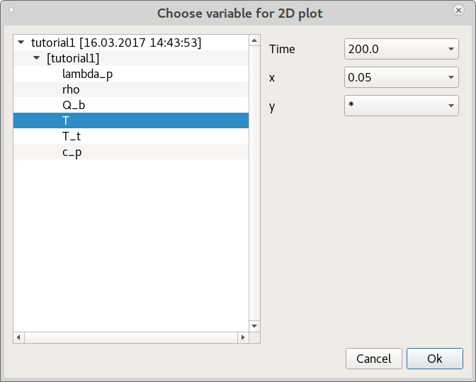
2D plots can be saved as templates (.pt files) which store the information in JSON format.

{
  "curves": [
      [
      "tutorial4.T",
      [
          -1
      ],
      [
          "*"
      ],
      "tutorial4.T(*)",
      {
          "color": "black",
          "linestyle": "-",
          "linewidth": 0.5,
          "marker": "o",
          "markeredgecolor": "black",
          "markerfacecolor": "black",
          "markersize": 6
      }
      ]
  ],
  "gridOn": true,
  "legendOn": true,
  "plotTitle": "",
  "updateInterval": 0,
  "windowTitle": "tutorial4.T(*)",
  "xlabel": "Time (s)",
  "xmax": 525.0,
  "xmax_policy": 0,
  "xmin": -25.0,
  "xmin_policy": 0,
  "xscale": "linear",
  "xtransform": 1.0,
  "ylabel": "T (K)",
  "ymax": 361.74772465755922,
  "ymax_policy": 1,
  "ymin": 279.2499308975365,
  "ymin_policy": 1,
  "yscale": "linear",
  "ytransform": 1.0,
}

6.10. Executing simulations

6.10.1. Initialising domains and parameters

Domains and parameters are initialised in the SetUpParametersAndDomains() function. In the case of deep model hierarchies domains and parameters having identical names can be initialised using the propagation technique and PropagateDomain() and PropagateParameter() functions. These functions traverse down all models in the hierarchy (starting with the calling model) and copy the properties of the given domain/parameter to all domains/properties with the same name.

6.10.2. Initialising variables (initial conditions, degrees of freedom)

All information related to variables are set in the SetUpVariables() function. Here, operations such as setting initial conditions, initial guesses, absolute tolerances and fixing degrees of freedom can be performed.

There are two initial condition modes supported by the Sundials IDAS solver (daeeInitialConditionMode):

• eAlgebraicValuesProvided (the default)

  Initial conditions are set using the SetInitialCondition() function.

• eQuasiSteadyState

  DAE solver assumes all derivatives to initially be zero (thus the name Quasi Steady State).

The initial condition mode can be set using the InitialConditionMode property (during the initialisation of the system in the SetUpVariables() function).

The initial conditions for Finite Element models are set in a different way (due to a nature of the block matrices used). Here, the function setFEInitialConditions() is used. It accepts the following arguments:

• FEmodel is an instance of daeFiniteElementModel class

• FEsystem is an instance of daeFiniteElementObject_t class (i.e. dealiiFiniteElementSystem_2D)

• dofName is a string with the dof name

• ic can be a float value or a callable that returns a float value for the given arguments: index_in_the_domain and overall_index

def SetUpVariables(self):
    setFEInitialConditions(self.m.fe_model, self.m.fe_system, 'T', 300.0)

6.10.3. Developing schedules (operating procedures)

The model specified in the simulation constructor is integrated in time in the Run() function. The default implementation iterates over the specified time horizon (TimeHorizon property), integrates for time intervals specified using the ReportingInterval property and reports the data. If a discontinuity occurs during the current integration interval, the precise discontinuity time is determined, model integrated until the discontinuity time point, data reported, the DAE system reinitialised and integration resumed.

The user-defined schedule can be implemented by overloading the Run() function. Here, a custom schedule can be specified using the following functions from the daeSimulation class:

• Integrate() integrates the system until the given time horizon is reached and reports the data after every reporting interval. If the stopCriterion argument is set to eStopAtModelDiscontinuity the simulation will be stopped at every discontinuity occurrence and if the reportDataAroundDiscontinuities argument is set to True the data reported at the discontinuity and after the system is reinitialised. The default value for reportDataAroundDiscontinuities is True. The condition that triggered the discontinuity can be retrieved using the LastSatisfiedCondition property which returns the daeCondition object.

• IntegrateForTimeInterval() integrates the system for the given time interval (in seconds). Its behaviour can be controlled using the stopCriterion and reportDataAroundDiscontinuities arguments in the same way as in the Integrate() function.

• IntegrateUntilTime() integrates the system until the specified time is reached (in seconds). Its behaviour can be controlled using the stopCriterion and reportDataAroundDiscontinuities arguments in the same way as in the Integrate() function.

• IntegrateForOneStep() integrates the system for a single time step (DAE solver dependent) Its behaviour can be controlled using the stopCriterion and reportDataAroundDiscontinuities arguments in the same way as in the Integrate() function.

• ReportData() reports the data at the current time in simulation.

• The functions ReSetInitialCondition() and ReAssignValue() can be used to re-set the initial conditions and re-assign the values of degrees of freedom. These calls must be followed by a call to the ReInitialize() function to reinitialise the system after the variable values have been modified.

The functionality of the default Run() function is roughly identical to the following python code:

def Run(self):
    # Python implementation of daeSimulation::Run() C++ function.

    import math
    while self.CurrentTime < self.TimeHorizon:
        # Get the time step (based on the TimeHorizon and the ReportingInterval).
        # Do not allow to get past the TimeHorizon.
        t = self.NextReportingTime
        if t > self.TimeHorizon:
            t = self.TimeHorizon

        # If the flag is set - a user tries to pause the simulation, therefore return.
        if self.ActivityAction == ePauseActivity:
            self.Log.Message("Activity paused by the user", 0)
            return

        # If a discontinuity is found, loop until the end of the integration period.
        # The data will be reported around discontinuities!
        while t > self.CurrentTime:
            self.Log.Message("Integrating from [%f] to [%f] ..." % (self.CurrentTime, t), 0)
            self.IntegrateUntilTime(t, eStopAtModelDiscontinuity, True)

        # After the integration period, report the data.
        self.ReportData(self.CurrentTime)

        # Set the simulation progress.
        newProgress = math.ceil(100.0 * self.CurrentTime / self.TimeHorizon)
        if newProgress > self.Log.Progress:
            self.Log.Progress = newProgress

A very simple schedule can be found in the Tutorial 7:

# The schedule:
#  1. Re-assign the value of Qin to 500W. After re-assigning DOFs or re-setting initial conditions
#     the function daeSimulation.Reinitialize() has to be called to reinitialise the DAE system.
#     Run the simulation for 100s using the function daeSimulation.IntegrateForTimeInterval()
#     and report the data using the function daeSimulation.ReportData().
#  2. Re-assign the value of Qin to 750W and re-initialise the system.
#     Use the function daeSimulation.IntegrateUntilTime() to run until the time reaches 200s
#     and report the data.
#  3. Re-assign the variable Qin to 1000W and re-initialise the system.
#     Use the function daeSimulation.IntegrateForOneStep() to integrate in OneStep mode for 100s
#     and report the data at every time step.
#  4. Re-assign the variable Qin to 1500W, re-set T to 300K and re-initialise the system.
#     Run the simulation until the TimeHorizon is reached using the function
#     daeSimulation.Integrate() and report the data.
def Run(self):
    # 1. Set Qin=500W and integrate for 100s
    self.m.Qin.ReAssignValue(500 * W)
    self.Reinitialize()
    self.ReportData(self.CurrentTime)
    self.Log.Message("OP: Integrating for 100 seconds ... ", 0)
    time = self.IntegrateForTimeInterval(100, eDoNotStopAtDiscontinuity)
    self.ReportData(self.CurrentTime)
    self.Log.SetProgress(int(100.0 * self.CurrentTime/self.TimeHorizon))

    # 2. Set Qin=750W and integrate until time = 200s
    self.m.Qin.ReAssignValue(750 * W)
    self.Reinitialize()
    self.ReportData(self.CurrentTime)
    self.Log.Message("OP: Integrating until time = 200 seconds ... ", 0)
    time = self.IntegrateUntilTime(200, eDoNotStopAtDiscontinuity)
    self.ReportData(self.CurrentTime)
    self.Log.SetProgress(int(100.0 * self.CurrentTime/self.TimeHorizon))

    # 3. Set Qin=1000W and integrate in OneStep mode for 100 seconds.
    self.m.Qin.ReAssignValue(1000 * W)
    self.Reinitialize()
    t_end = time + 100.0
    self.Log.Message("OP: Integrating in one step mode:", 0)
    while time < t_end:
        msg = "    Integrated from %.10f to " % time
        time = self.IntegrateForOneStep(eDoNotStopAtDiscontinuity)
        self.ReportData(self.CurrentTime)
        msg += "%.10f ... " % time
        self.Log.Message(msg, 0)

    # 4. Set Qin=1500W and integrate until the specified TimeHorizon is reached
    self.m.Qin.ReAssignValue(1500 * W)
    self.m.T.ReSetInitialCondition(300 * K)
    self.Reinitialize()
    self.ReportData(self.CurrentTime)
    self.Log.SetProgress(int(100.0 * self.CurrentTime/self.TimeHorizon))
    self.Log.Message("OP: Integrating from " + str(time) + " to the time horizon (" + str(self.TimeHorizon) + ") ... ", 0)
    time = self.Integrate(eDoNotStopAtDiscontinuity)
    self.ReportData(self.CurrentTime)
    self.Log.SetProgress(int(100.0 * self.CurrentTime/self.TimeHorizon))
    self.Log.Message("OP: Finished", 0)

In addition, the Advanced Tutorial 1 illustrates interactive schedules where the pyQt graphical user interface (GUI) is utilised to manipulate the model variables and integrate the system in time:

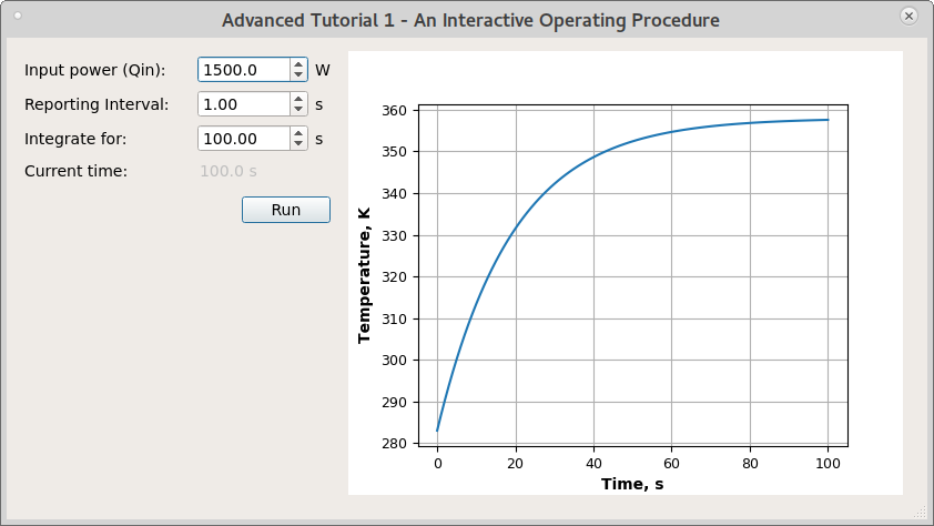
6.10.4. Exploring models using the GUI (Simulation Explorer)

The model structure and the domains/parameters/variables data can be interactively explored and updated using the Simulation Explorer GUI. The Simulation Explorer can be started using the following code:

...
# Create and initialize the simulation and the auxiliary objects and
# determine the consistent initial conditions using the SolveInitial function.
...
simulation.SolveInitial()

# Show the simulation explorer GUI
app = daeCreateQtApplication(sys.argv)
se = daeSimulationExplorer(app, simulation)
se.exec_()

or from the DAE Toools Simulator Start/Show simulation explorer ad run… button:

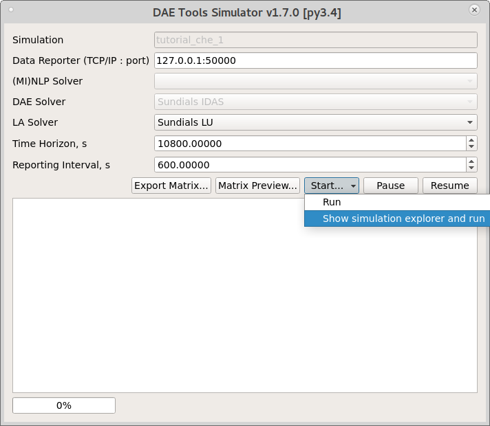
Screenshots of the running Simulation Explorer:

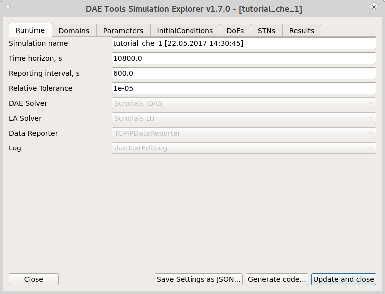
Fig. 6.3 Runtime simulation options

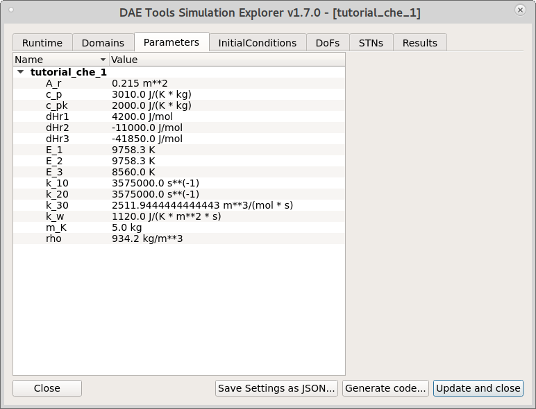
Fig. 6.4 Parameters values

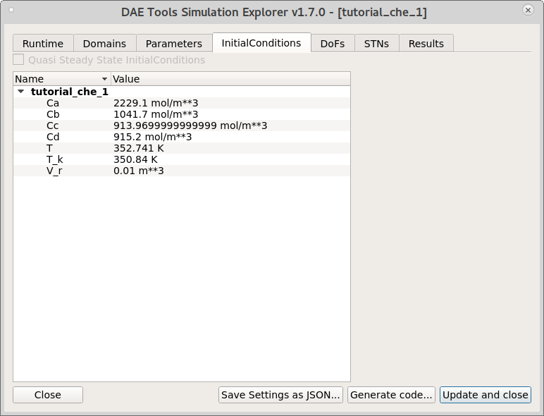
Fig. 6.5 Initial conditions

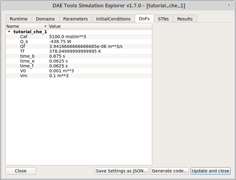
Fig. 6.6 Degrees of freedom

6.11. Parallel computation

Within the DAE Tools only the shared-memory parallel programming model is supported. Simulation on message-passing systems is available through the OpenCS code generator (section Generating code for other modelling languages). The following parts of the code support parallelisation.

6.11.1. Evaluation of equations

Equations residuals, Jacobian matrix and sensitivity residuals can be evaluated in parallel using two methods:

1. The Evaluation Tree approach (default)

   Equations are transformed using the operator overloading technique into a tree-like data structure called an Evaluation Tree. For instance, it is already shown that the equation \(\frac{x[0]-x[1]} {x[2]-x[3]} + 1.2 \cdot sin(x[0]) = 0\) can be represented as:

   

   Equations can be evaluated in parallel using OpenMP API. This evaluation mode is specified in the section daetools.core.equations of daetools.cfg config file by setting the evaluationMode option to “evaluationTree_OpenMP”. If numThreads is 0 the default number of threads is used (the number of cores in the system). Sequential evaluation is achieved by setting numThreads to 1.

2. The Compute Stack approach

   Equations are transformed using the operator overloading technique into a postfix notation expression stacks. Each operand/operation is described by the specially designed data structure, and every equation is transformed into an array of these structures (a Compute Stack). Compute Stacks are evaluated by a stack machine using a FIFO queue. As an example, the equation above can also be represented as a Compute Stack:

   

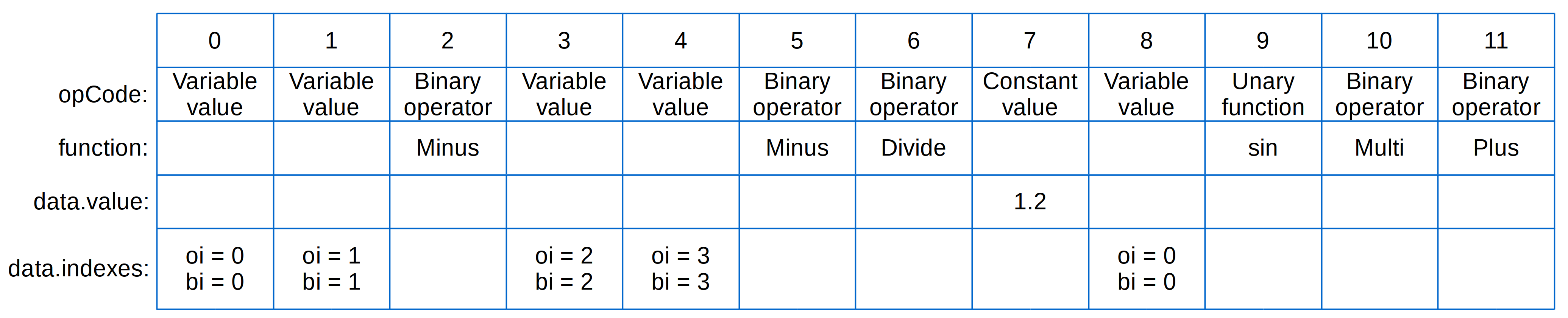
   Equations can be evaluated in parallel using:

   1. OpenMP API for general purpose processors and manycore devices (i.e. Xeon Phi)

      This evaluation mode is specified in the section daetools.core.equations of daetools.cfg config file by setting the evaluationMode option to “computeStack_OpenMP”. If numThreads is 0 the default number of threads is used (the number of cores in the system). Sequential evaluation is achieved by setting numThreads to 1.

   2. OpenCL framework for streaming processors (GPU, GPGA) and heterogeneous systems

      This type is implemented in an external Python module pyEvaluator_OpenCL. It is up to one order of magnitude faster than the Evaluation Tree approach. However, it does not support external functions nor thermo-physical packages.

      It is required to install OpenCL drivers/runtime libraries. Good starting points for different hardware vendors could be:

      • InteL: https://software.intel.com/en-us/articles/opencl-drivers

      • AMD: https://support.amd.com/en-us/kb-articles/Pages/OpenCL2-Driver.aspx

      • NVidia: https://developer.nvidia.com/opencl

      The available OpenCL platforms and devices can be listed using AvailableOpenCLPlatforms() and AvailableOpenCLDevices() functions:

      from daetools.pyDAE.evaluator_opencl import pyEvaluator_OpenCL
      
      openclPlatforms = pyEvaluator_OpenCL.AvailableOpenCLPlatforms()
      openclDevices   = pyEvaluator_OpenCL.AvailableOpenCLDevices()
      

      A sample list of available OpenCL platforms and devices (from Tutorial 21) are presented below:

      Available OpenCL platforms:
          Platform: NVIDIA CUDA
              PlatformID: 0
              Vendor:     NVIDIA Corporation
              Version:    OpenCL 1.2 CUDA 9.0.194
      
          Platform: Intel(R) OpenCL
              PlatformID: 1
              Vendor:     Intel(R) Corporation
              Version:    OpenCL 2.0
      
      Available OpenCL devices:
          Device: GeForce GTX 950M
              PlatformID:      0
              DeviceID:        0
              DeviceVersion:   OpenCL 1.2 CUDA
              DriverVersion:   384.90
              OpenCLVersion:   OpenCL C 1.2
              MaxComputeUnits: 5
      
          Device: Intel(R) HD Graphics
              PlatformID:      1
              DeviceID:        0
              DeviceVersion:   OpenCL 2.0
              DriverVersion:   r5.0.63503
              OpenCLVersion:   OpenCL C 2.0
              MaxComputeUnits: 24
      
          Device: Intel(R) Core(TM) i7-6700HQ CPU @ 2.60GHz
              PlatformID:      1
              DeviceID:        1
              DeviceVersion:   OpenCL 2.0 (Build 475)
              DriverVersion:   1.2.0.475
              OpenCLVersion:   OpenCL C 2.0
              MaxComputeUnits: 8
      

      External Compute Stack Evaluators are set using daeSimulation.SetComputeStackEvaluator() function:

      from daetools.pyDAE.evaluator_opencl import pyEvaluator_OpenCL
      
      # OpenCL evaluators can use a single or multiple OpenCL devices.
      #   a) Single OpenCLdevice:
      evaluator = pyEvaluator_OpenCL.CreateComputeStackEvaluator(platformID = 0, deviceID = 0)
      
      #   b) Multiple OpenCL devices (for heterogenous computing):
      #      They require the platformID, deviceID and percentage of the total work
      #      to be specified for each device.
      evaluator = pyEvaluator_OpenCL.CreateComputeStackEvaluator( [(0, 0, 60), (1, 1, 40)] )
      
      simulation.SetComputeStackEvaluator(evaluator)
      

6.11.2. Assembly of Finite Element systems

Assembly of Finite Element matrices can be performed in parallel using OpenMP API. The options are located in the daetools.cfg config file, section daetools.deal_II.assembly. The parallel assembly can be switched on by setting the parallelAssembly option. parallelAssembly can be Sequential or OpenMP. If numThreads is 0 the default number of threads will be used (typically the number of cores in the system). The queueSize specifies the size of the internal queue; when this size is reached the local data are copied to the global matrices.

6.11.3. Solution of systems of linear equations

The following multi-threaded linear solvers are supported: SuperLU_MT, Pardiso and Intel Pardiso.

6.11.4. Global Sensitivity Analysis

Simulations can be performed using multiprocessing.Pool available in Python.

6.12. DAE Tools web services

Simulations can be loaded and executed using the Representational state transfer (REST) web service. RESTful API is provided for almost complete daeSimulation functionality (daetools_ws) and for all FMI v2 for co-simulation functions (daetools_fmi_ws). The RESTful API is language-independent and can be used from any language (i.e. JavaScript, Python, C++ …).

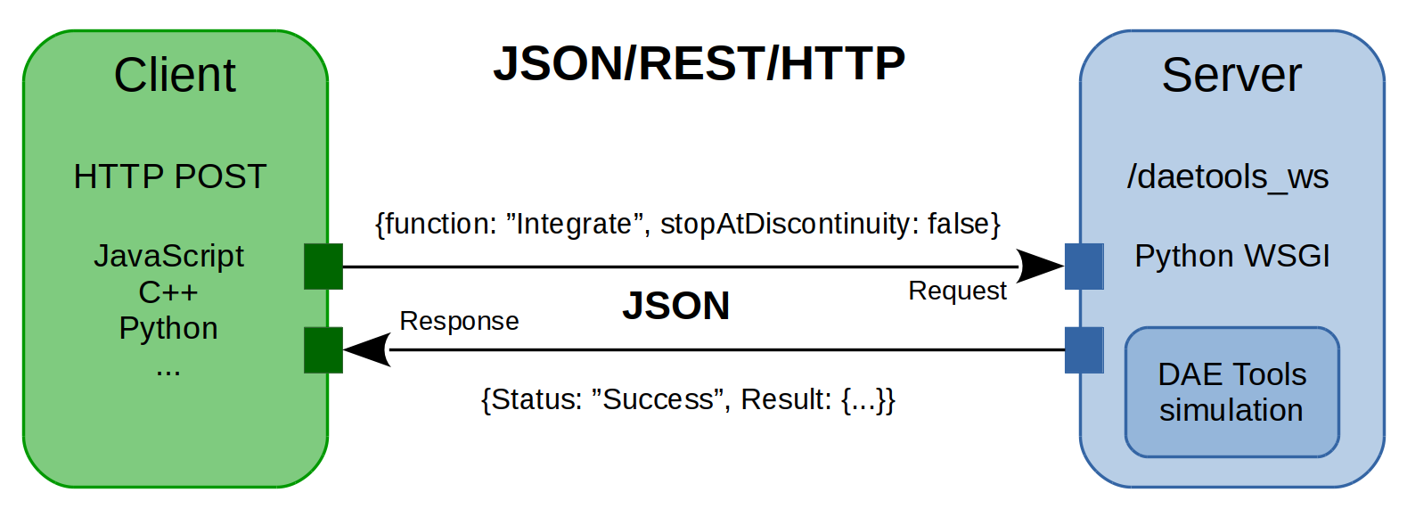
Fig. 6.7 REST web service

Web services can be started using the following commands:

# DAE Tools simulations web service.
# By default, starts the web service on the "localhost" (http://127.0.0.1:8001)
python -m daetools.dae_simulator.daetools_ws

# Individual simulations as a web service.
# Add the simulation names to the 'availableSimulations' dictionary and start the service.
# The loaderFunction is a Python callable object that returns an initialised simulation object
# and will be called when a client requests a simulation by name.
availableSimulations = {}
availableSimulations['tutorial_che_1']  = loaderFunction
daeSimulationWebService.runSimulationsAsWebService(availableSimulations)

# FMI v2 web service.
# By default, starts the web service on the "localhost" (http://127.0.0.1:8002)
python -m daetools.dae_simulator.daetools_fmi_ws

JavaScript client classes are developed for both types of web services. Classes are located in the daetools/dae_simulator folder. web_service.js contains the web service client, daetools_ws.js contains daeSimulation interface and daetools_fmi_ws.js contains FMI interface.

JavaScript client interface for daetools_ws simulations web service:

class daeSimulation
{
    LoadSimulation(pythonFile, loadCallable, args);
    LoadTutorial(tutorialName);
    LoadSimulationByName(simulationName, args);
    AvailableSimulations();
    Finalize();
    get ModelInfo();
    get Name();
    get DataReporter();
    get DAESolver();
    get CurrentTime();
    get TimeHorizon();
    set TimeHorizon(timeHorizon);
    get ReportingInterval();
    set ReportingInterval(reportingInterval);
    Run();
    SolveInitial();
    Reinitialize();
    Reset();
    ReportData();
    Integrate(stopAtDiscontinuity, reportDataAroundDiscontinuities);
    IntegrateForTimeInterval(timeInterval, stopAtDiscontinuity, reportDataAroundDiscontinuities);
    IntegrateUntilTime(time, stopAtDiscontinuity, reportDataAroundDiscontinuities);
    GetParameterValue(name);
    GetVariableValue(name);
    GetActiveState(stnName);
    SetParameterValue(name, value);
    ReAssignValue(name, value);
    ReSetInitialCondition(name, value);
    SetActiveState(stnName, activeState);
}

JavaScript client interface for daetools_fmi_ws FMI web service:

class daeFMI2Simulation
{
    fmi2Instantiate(instanceName, guid, resourceLocation);
    fmi2Terminate();
    fmi2FreeInstance();
    fmi2SetupExperiment(toleranceDefined, tolerance, startTime, stopTimeDefined, stopTime);
    fmi2EnterInitializationMode();
    fmi2ExitInitializationMode();
    fmi2Reset();
    fmi2DoStep(currentCommunicationPoint, communicationStepSize, noSetFMUStatePriorToCurrentPoint);
    fmi2CancelStep();
    fmi2GetReal(valReferences);
    fmi2SetReal(valReferences, values);
    fmi2GetString(valReferences);
    fmi2SetString(valReferences, values);
    fmi2GetBoolean(valReferences);
    fmi2SetBoolean(valReferences, values);
    fmi2GetInteger(valReferences);
    fmi2SetInteger(valReferences, values);
}

A sample simulation in JavaScript is given in the following listing:

// Create the web service client.
var webService = new daeWebService('127.0.0.1', 8001, 'daetools_ws');

// Create the simulation object.
var simulation = new daeSimulation(webService);

// Load simulation by name (if it has been started as a web service):
simulation.LoadSimulationByName('simulationName', JSON.stringify(args));
// or load one of tutorials:
simulation.LoadTutorial('tutorialName');
// or load simulation by specifying a path to Python file, loading function and its arguments:
simulation.LoadSimulation('pythonFile', 'loadCallable', args)

var reportingInterval = simulation.ReportingInterval;
var timeHorizon       = simulation.TimeHorizon;
var currentTime       = simulation.CurrentTime;

// Get the consistent initial conditions.
simulation.SolveInitial();

// Integrate the system in a loop until the time horizon is reached.
while(currentTime < timeHorizon)
{
    // Get the next time (based on the TimeHorizon and the ReportingInterval).
    // Do not allow to get past the TimeHorizon.
    var t = currentTime + reportingInterval;
    if(t > timeHorizon)
        t = timeHorizon;

    // If a discontinuity is found, loop until the end of the integration period.
    // The data will be reported around discontinuities!
    while(t > currentTime)
    {
        log('Integrating from ' + currentTime.toFixed(2) + ' to ' + t.toFixed(2) + ' ...');
        currentTime = simulation.IntegrateUntilTime(t, true, true);
    }

    // After the integration period, report the data.
    simulation.ReportData()

    // Set the simulation progress.
    var newProgress = Math.ceil(100.0 * currentTime / timeHorizon)
    setProgress(newProgress);
}

// Clean up.
simulation.Finalize();

Calls to the above functions translate to HTTP requests. For instance, a call to simulation.IntegrateUntilTime(100.0, true, true) results in a HTTP request sent to the daetools_ws web service: http://127.0.0.1:8001/daetools_ws?simulationID=ba2a694a-b591-11e7-9f58-680715e7b846&function=IntegrateUntilTime&time=100.0&stopAtDiscontinuity=true&reportDataAroundDiscontinuities=true. The response is returned in JSON format.

Sample html pages with the Graphical User Interface (GUI) using JavaScript and Plotly.js library are provided for both types of web services and presented in figure below. Web pages are located in the daetools/dae_simulator folder: daetools_ws_test.html and daetools_fmi_ws_test.html.

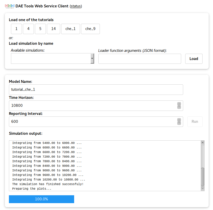
Fig. 6.8 HTML+JavaScript GUI for daetools_ws web service client

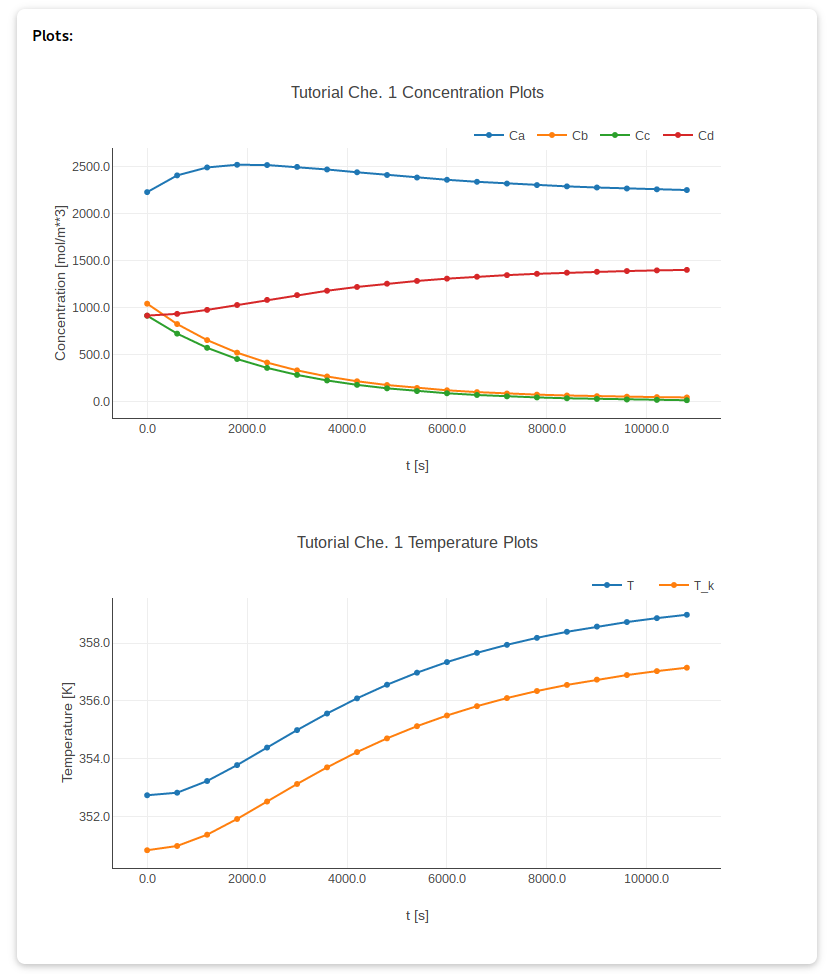
Fig. 6.9 Plots produced by HTML GUI for daetools_ws web service client using Plotly.js library

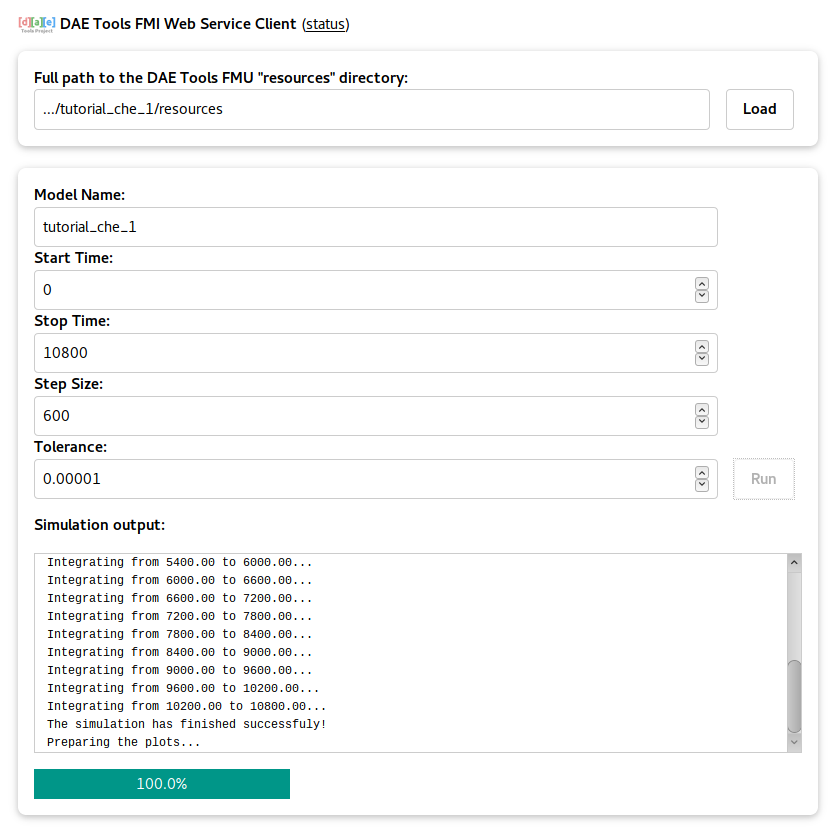
Fig. 6.10 HTML+JavaScript GUI for daetools_fmi_ws web service client

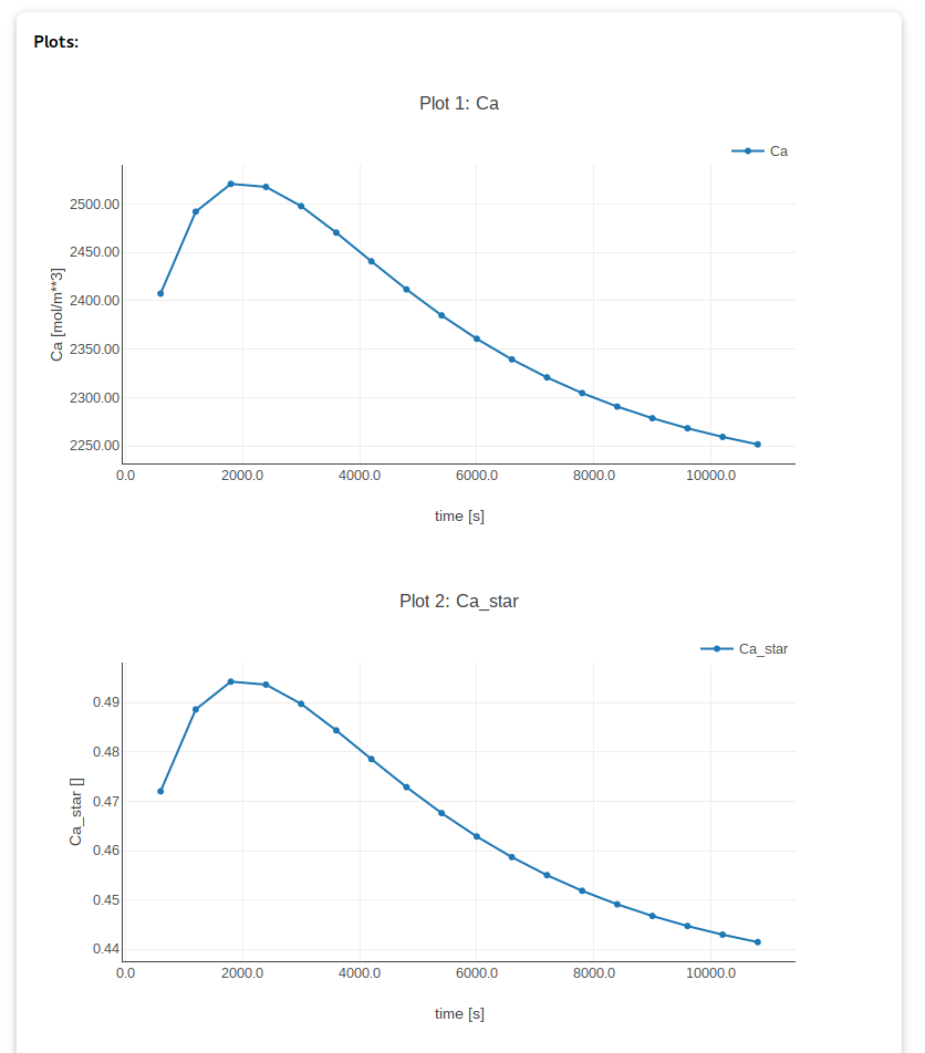
Fig. 6.11 Plots produced by daetools_fmi_ws web service client using Plotly.js library

6.13. Generating code for other modelling languages

DAE Tools can generate code for several modelling or programming languages (Modelica, gPROMS, c99, OpenCS). The code generation should be performed after the simulation is initialised (ideally after a call to SolveInitial() so that the consistent initial conditions are determined and available).

# Generate Modelica source code:
from daetools.code_generators.modelica import daeCodeGenerator_Modelica
cg = daeCodeGenerator_Modelica()
cg.generateSimulation(simulation, tmp_folder)

# Generate gPROMS source code:
from daetools.code_generators.gproms import daeCodeGenerator_gPROMS
cg = daeCodeGenerator_gPROMS()
cg.generateSimulation(simulation, tmp_folder)

# Generate OpenCS models to be simulated using MPI on 4 nodes:
from daetools.code_generators.opencs import daeCodeGenerator_OpenCS
cg = daeCodeGenerator_OpenCS()
cg.generateSimulation(simulation, tmp_folder, 4)

The generateSimulation() function requires an initialised simulation object and the directory where the code will be generated.

The code can be also generated from the Generate code… option in the Simulation Explorer GUI:

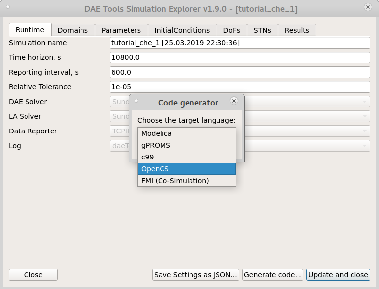
Fig. 6.12 Code generation from the Simulation Explorer GUI

More details can be found in Advanced Tutorial 3 and Advanced Tutorial 4.

6.14. Simulating models in other simulators (co-simulation)

DAE Tools can also wrap the models developed in python for use in other software/simulators: FMI (Functional Mock-up Interface for co-simulation), Matlab, Scilab and GNU Octave MEX functions, and Simulink S-functions.

6.14.1. Functional Mock-up Interface for co-simulation (FMI)

DAE Tools models can be used to generate .fmu files for FMI for co-simulation.

Nota bene

The model inputs are defined by the inlet ports while the model outputs by the outlet ports. In addition, assigned variables (degrees of freedom) from the top-level model are added to the list of inputs and the rest of variables from the top-level model can be added as either local FMI variables or as outputs.

Generating FMU files for use in FMI capable simulators is similar to the code-generation procedure. The generateSimulation() function generates a simulation name.fmu file which is basically a zip file with the files required by the FMI standard. Here, the generateSimulation() function requires the following arguments:

• simulation: initialised daeSimulation object

• directory: directory where the .fmu file will be generated

• py_simulation_file: a path to the python file with the simulation source code

• create_simulation_callable_object: the name of python callable object that returns an initialized daeSimulation object

• arguments: arguments for the above callable object; can be anything that python accepts

• additional_files: paths to the additional files to pack into a .fmu file (empty list by default)

• localsAsOutputs: if True all variables from the top-level model will be treated as model outputs, otherwise as locals

• add_xml_stylesheet: if True the xsl file daetools-fmi.xsl will be added to the modelDescription.xml file

• useWebService: if True the web service version (fmi_ws) shared library will be packed into the fmu file. DAE Tools FMI web service can be started using: python -m daetools.dae_simulator.daetools_fmi_ws. The fmu will attempt to start it automatically and connect during the initialisation phase.

All tutorials provide run(**kwargs) function that can be used to run a simulation (using the console or Qt GUI) and for co-simulation to return an initialised simulation object (if the initializeAndReturn argument is True). This way the same setup can be used for different activities.

from daetools.code_generators.fmi import daeCodeGenerator_FMI
cg = daeCodeGenerator_FMI()
cg.generateSimulation(simulation,
                      directory            = tmp_folder,
                      py_simulation_file   = __file__,
                      callable_object_name = 'run',
                      arguments            = 'initializeAndReturn = True',
                      additional_files     = [],
                      localsAsOutputs      = True,
                      add_xml_stylesheet   = True)

In addition, the create_simulation_callable_object argument can be any other user-defined function (as specified in the Advanced Tutorial 3 example):

# This function is used by daetools_mex, daetools_s and daetools_fmi_cs to load a simulation.
# It can have any number of arguments, but must return an initialized daeSimulation object.
def create_simulation():
    # Create Log, Solver, DataReporter and Simulation object
    log          = daePythonStdOutLog()
    daesolver    = daeIDAS()
    datareporter = daeNoOpDataReporter()
    simulation   = simTutorial()

    # Enable reporting of all variables
    simulation.m.SetReportingOn(True)

    # Set the time horizon and the reporting interval
    simulation.ReportingInterval = 1
    simulation.TimeHorizon       = 100

    # Initialize the simulation
    simulation.Initialize(daesolver, datareporter, log)

    return simulation

6.14.2. MEX functions

In order to simulate DAE Tools models from Matlab/Scilab/GNU Octave the wrapper code first needs to be compiled from source. The wrapper code is located in the daetools/trunk/mex directory. The compilation procedure requires a compiled cdaeSimulationLoader-py[Major][(Minor] library (which is a part of DAE Tools installation) located in the daetools/solibs/Platform_Architecture directory (i.e. daetools/solibs/Windows_win32). That directory has to be made available to the mex compiler and Matlab during runtime:

1. Set environmental variable LD_LIBRARY_PATH in Matlab (using the setenv and getenv commands)

2. Set RPATH in the mex file during the linking procedure

For instance, setting the LD_LIBRARY_PATH environmental variable can be done with the following code:

% Note the path separator (; or :)
% Windows
setenv('LD_LIBRARY_PATH', [getenv('LD_LIBRARY_PATH') ';path to daetools/solibs directory']);
% GNU/Linux
setenv('LD_LIBRARY_PATH', [getenv('LD_LIBRARY_PATH') ':path to daetools/solibs directory']);

Compilation from Matlab (for python 2.7):

cd mex
mex -v -I../simulation_loader -lcdaeSimulationLoader-py27 daetools_mex.c

Compilation from GNU Octave (for python 2.7):

cd mex
mkoctfile -v --mex -I../simulation_loader -lcdaeSimulationLoader-py27 daetools_mex.c

Compilation from Scilab (for python 2.7):

cd mex
# check the include flag: cflags = -I... and set the correct full path for simulation loader
exec('builder.sce')
exec('loader.sce')

Now the compiled daetools_mex executable can be used to run DAE Tools simulations from Matlab:

res = daetools_mex('.../daetools/examples/tutorial_adv_3.py', 'create_simulation', ' ', 100.0, 10.0)

daetools_mex accepts the following arguments:

1. Path to the python file with daetools simulation (char array)

2. The name of python callable object that returns an initialized daeSimulation object (char array)

3. Arguments for the above callable object; can be anything that python accepts (char array)

4. Time horizon (double scalar)

5. Reporting interval (double scalar)

The outputs from the daetools_mex MEX-function are:

1. Cell array (pairs: {‘variable_name’, double matrix}). The variables values are put into the caller’s workspace as well.

6.14.3. Simulink S-functions

Again, in order to simulate DAE Tools models from Simulink the wrapper code first needs to be compiled from source. The wrapper code is located in the daetools/trunk/mex directory. The compilation procedure requires a compiled cdaeSimulationLoader-py[Major][(Minor] library (which is a part of DAE Tools installation) located in the daetools/solibs/Platform_Architecture directory (i.e. daetools/solibs/Windows_win32). That directory has to be made available to the mex compiler and Matlab during runtime as explained in the MEX functions section.

Compilation from Simulink (for python 2.7):

cd mex
mex -v -I../simulation_loader  -lcdaeSimulationLoader-py27 daetools_s.c

Running deatools_s S-functions:

• Add a new S-Function (‘system’) from the User-Defined Functions palette.

• Set its dialog box parameters:

  • S-Function name: daetools_s (this is a compiled daetools_s.c file, resulting in, for instance, deatools_s.mexa64 binary)

  • S-Function parameters: see the description below

    example: ‘…/daetools/examples/tutorial_adv_3.py’, ‘create_simulation’, ‘ ‘, 2, 2

  • S-Function modules: leave blank

As a working example, the file test_s_function.mdl in daetools/trunk/mex directory can be used.

deatools_s S-function parameters:

1. Path to the python file with daetools simulation (char array)

2. The name of python callable object that returns initialized daeSimulation object (char array)

3. Arguments for the above callable object; can be anything that python accepts (char array)

4. Number of input ports (integer, must match the number of inlet ports in daetools simulation)

5. Number of output ports (integer, must match the number of outlet ports in daetools simulation)

More details can be found in Advanced Tutorial 3.

6.15. Performing sensitivity analysis

Sensitivity analysis (SA) is the study of how the uncertainty in the output of a mathematical model or system (numerical or otherwise) can be apportioned to different sources of uncertainty in its inputs [4]. Sensitivity analysis is conducted to [4] [5]:

1. Identify the most important parameters (those that contribute the most to output variability)

2. Identify insignificant parameters (can be eliminated from the model)

3. Determine if and which parameters interact with each other

4. Simplify the model (by fixing model inputs that have no effect on the output)

5. Test the robustness of a model in the presence of uncertainty

6. Detect errors in the model (by encountering unexpected relationships between inputs and outputs)

7. Reduce uncertainty through the identification of model inputs that cause significant uncertainty in the output

8. Determine the optimal regions within the parameters space (for use in optimisation studies)

There is a large number of SA methods, but in general they can be grouped into the local and global methods. The local methods involve calculation of the partial derivatives of the output with respect to an input factor. The most important local (derivative-based) methods are:

• Forward sensitivity method

• Adjoint sensitivity method

The global methods can be grouped into:

• The screening methods (coarse sorting of the most influential inputs among a large number, such as Morris Elementary Effects method)

• The measures of importance (quantitative sensitivity indices)

• The variance-based methods for deep exploration of the model behaviour (measuring the effects of inputs on their all variation range, such as FAST, Sobol)

Other methods include One-at-a-time (changing one-factor-at-a-time to determine the effect on the output), Regression analysis and Scatter plots (scatter plots of the output variable against individual input variables, after sampling the model over its input distributions).

DAE Tools support both local and global sensitivity analysis methods. The local derivative-based method utilises Sundials IDAS sensitivity analysis capabilities to determine the sensitivity of the results with respect to the model parameters. At the moment, only the forward sensitivity method is available. The global SA can be performed using the external libraries (i.e. SALib).

6.15.1. Local (derivative-based) SA methods

To enable integration of sensitivity equations the function Initialize() must be called with the calculateSensitivities argument set to true:

simulation.Initialize(daesolver, datareporter, log, calculateSensitivities = True)

and the model parameters specified in the SetUpSensitivityAnalysis() function using the SetSensitivityParameter() method:

def SetUpSensitivityAnalysis(self):
    self.SetSensitivityParameter(variable_1)
    ...
    self.SetSensitivityParameter(variable_n)

Nota bene

The sensitivity parameters must be variables with the assigned value (degrees of freedom)!

Sensitivities can be reported to a data reporter like any ordinary variable by setting the boolean property ReportSensitivities to True. In this case, the sensitivities for the variable var per parameter param are reported as sensitivities.d(var)_d(param).

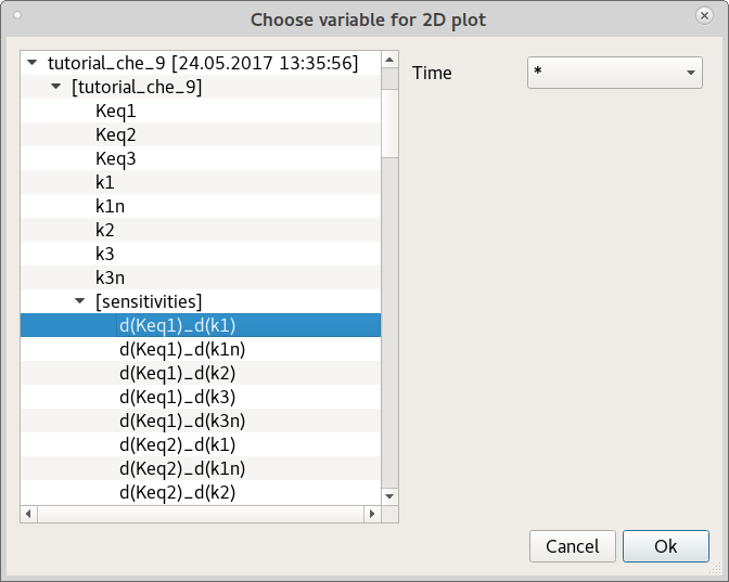
In addition, they can be obtained directly from the DAE solver after every call to Integrate() functions using the SensitivityMatrix property. This property returns a dense matrix as a daeDenseMatrix object. The numpy array object can be obtained from the daeDenseMatrix using the npyValues property.

More details on local sensitivity analysis methods can be found in Sensitivity Analysis Example 1, Sensitivity Analysis Example 2 and Chem. Eng. Example 9.

6.15.2. Global SA methods

Typically, the global sensitivity analysis is conducted by [4] [6]:

1. Defining the model and its input parameters and output variables

2. Assigning probability density functions to each input parameter

3. Generating an input matrix through an appropriate random sampling method, evaluating the output

4. Assessing the influences or relative importance of each input parameter on the output variable

An example of the global sensitivity analysis in DAE Tools is given in Sensitivity Analysis Example 3. This tutorial illustrates the global variance-based sensitivity analysis methods available in SALib python library. Three SA methods were applied on a thermal analysis of a batch reactor with exothermic reaction \(A \rightarrow B\) [6]: Morris (Elementary Effect method), FAST and Sobol (Variance-based methods).

In DAE Tools the procedure includes the following steps:

1. Selection of the global sensitivity method

2. Definition of the model inputs:

   SA_problem = {
     'num_vars': 5,
     'names': ['B', 'gamma', 'psi', 'theta_a', 'theta_0'],
     'bounds': [[10, 30],    # B
                [15, 25],    # gamma
                [0.4, 0.6],  # psi
                [-0.2, 0.2], # theta_a
                [-0.2, 0.2]  # theta_0
               ]
             }
   

3. Generation of samples:

   from SALib.sample.saltelli import sample
   
   # Generate samples using a Saltelli's extension of the Sobol sequence.
   # Sample size n=512, no. params k=5 => N=(2k+2)*n=6144 (as in the referenced article).
   param_values = sample(problem, 512, calc_second_order=True)
   

4. Generation of outputs for a given input matrix (by repeated simulations of a DAE Tools model):

   # theta_max is the analysed output from simulations
   # The function simulate() performs daetools simulation for a given set of input parameters
   theta_max  = numpy.zeros(N)
   for i in range(N):
       theta_max[i] = simulate(run_no  = i,
                               n       = 1,
                               B       = B[i],
                               gamma   = gamma[i],
                               psi     = psi[i],
                               theta_a = theta_a[i],
                               x_0     = 0.0,
                               theta_0 = theta_0[i])
   

   Calculations can also be performed in parallel:

   from multiprocessing import Pool
   # Create a pool of workers to calculate N outputs
   # Don't forget to disable OpenMP for evaluation of residuals and derivatives!!
   pool = Pool()
   args = [(i, 1, B[i], gamma[i], psi[i], theta_a[i], 0.0, theta_0[i]) for i in range(N)]
   theta_max[:] = pool.map(simulate_p, args, chunksize=1)
   

   Whether the simulations will be performed in parallel depends on model complexity and size. Running several large simulations that require a lot of memory at the same time may actually slow down the overall progress. Those cases will benefit more from parallel evaluation of equations / use of multithreaded linear equations solvers.

5. Performing sensitivity analysis

   from SALib.analyze.sobol import analyze
   
   res = analyze(problem, theta_max, print_to_console=False)
   
   # 1st-order variance-based sensitivities and the confidence intervals
   # (individual parameters contributions)
   S1      = res['S1']
   S1_conf = res['S1_conf']
   
   # 2nd-order variance-based sensitivities and the confidence intervals
   # (interactions between parameters)
   S2      = res['S2']
   S2_conf = res['S2_conf']
   
   # Total sensitivity indices and the confidence intervals
   ST      = res['ST']
   ST_conf = res['ST_conf']
   

   1st order and total sensitivity indices (for the Sobol method):

   -------------------------------------------------------
       Param          S1    S1_conf         ST    ST_conf
   -------------------------------------------------------
           B    0.094110   0.089475   0.581946   0.150334
       gamma   -0.002416   0.011938   0.044354   0.028461
         psi    0.171040   0.097859   0.524576   0.140252
     theta_a    0.072511   0.043878   0.523382   0.177241
     theta_0    0.002343   0.004746   0.008174   0.007650
   

   2nd order sensitivities (for the Sobol method):

   -------------------------------------------------------
   Parameter pairs          S2    S2_conf
   -------------------------------------------------------
           B/gamma    0.180434   0.153318
             B/psi    0.260698   0.172012
         B/theta_a    0.143292   0.145452
         B/theta_0    0.177137   0.150218
         gamma/psi    0.000981   0.024855
     gamma/theta_a    0.004953   0.040380
     gamma/theta_0   -0.009390   0.027726
       psi/theta_a    0.166102   0.173568
       psi/theta_0   -0.016474   0.132210
   theta_a/theta_0    0.109086   0.112104
   

6. Generation of scatter plots (using matplotlib.pyplot.scatter() function):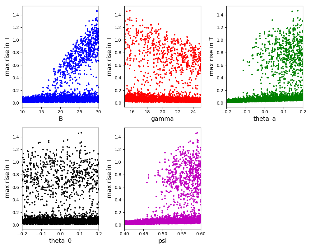

   

Footnotes

[4] (1,2,3)

A. Saltelli et al. Global sensitivity analysis. The Primer. Wiley-Interscience (2008). ISBN-10: 0470059974

[5]

D.J. Pannell. Sensitivity Analysis of Normative Economic Models: Theoretical Framework and Practical Strategies. Agricultural Economics 1997; 16:139–152. doi:10.1016/S0169-5150(96)01217-0

[6] (1,2)

A. Saltelli, M. Ratto, S. Tarantola, F. Campolongo. Sensitivity Analysis for Chemical Models. Chem. Rev. (2005), 105(7):2811-2828. doi:10.1021/cr040659d

6.16. Executing optimisations

The goal of mathematical optimisation is to select a best element (with regard to some criterion) from some set of available alternatives [7].

The following types of optimisation problems are supported in DAE Tools:

• Nonlinear optimisation problems

• Mixed-integer nonlinear programming

• Constrained and unconstrained problems

• Continuous and discrete problems

6.16.1. Optimisation setup

In general, the optimisation activities use the same model specification and the same simulation setup as in the simulation runs. However, some additional information are required:

1. The objective function

2. Optimisation variables

3. Optimisation constraints

These information are specified in the SetUpOptimization() function.

6.16.1.1. Specifying the objective function

By default, a single objective function object is declared and the objective function can be accessed using the ObjectiveFunction property. Its residual can be set as in ordinary equations. It is assumed that the optimisation solver tries to perform a minimisation. If a maximisation is required the objective function should be specified as \(-F_{obj}\).

def SetUpOptimization(self):
    # x1, x2 and x3 are optimisation variables (assigned variables, that is degrees of freedom).

    # The ObjectiveFunction object is automatically created by the framework
    # and only its residual needs to be specified.
    self.ObjectiveFunction.Residual = self.m.x1() + self.m.x2() + self.m.x3()

Scaling of the objective function can be left to be done by optimisation solvers or set manually. The default scaling is 1.0 and can be changed using the Scaling property. In addition, the objective function absolute tolerance can be specified using the AbsTolerance property.

6.16.1.2. Specifying optimisation variables

There are three types of optimisation variables in DAE Tools:

1. Continuous (specified using the function SetContinuousOptimizationVariable())

2. Integer (specified using the function SetIntegerOptimizationVariable())

3. Binary (value 0 or 1) (specified using the function SetBinaryOptimizationVariable())

def SetUpOptimization(self):
    # x1, x2 and x3 are optimisation variables (assigned variables, that is degrees of freedom).

    # Continuous optimisation variable: (lower bound, upper bound and the starting point as floats)
    self.ov1 = self.SetContinuousOptimizationVariable(self.m.x1, 0.0, 10.0, 1.5);

    # Integer optimisation variable: (lower bound, upper bound and the starting point as integers)
    self.ov2 = self.SetIntegerOptimizationVariable(self.m.x2, 1, 5, 2)

    # Binary optimisation variable: (the starting point)
    self.ov3 = self.SetBinaryOptimizationVariable(self.m.x3, 0)

6.16.1.3. Specifying optimisation constraints

There are three types of optimisation constraints in DAE Tools:

1. Inequality (specified using the function CreateInequalityConstraint())

2. Equality (specified using the function CreateEqualityConstraint())

Constraints in DAE Tools are similar to ordinary equations.

def SetUpOptimization(self):
    # x1, x2 and x3 are optimisation variables (assigned variables, that is degrees of freedom).

    # Inequality constraint: g(i) <= 0)
    # The constraint: x1 >= 25 in daetools becomes: 25 - x1 <= 0
    self.c1 = self.CreateInequalityConstraint("Constraint 1")
    self.c1.Residual = 25 - self.m.x1()

    # Equality constraint: h(i) = 0
    # The constraint: x2 + x3 = 10 in daetools becomes: x2 + x3 - 10 = 0
    self.c2 = self.CreateEqualityConstraint("Constraint 2")
    self.c2.Residual = self.m.x1() + self.m.x2() - 10

Scaling of constraints can be left to be done by optimisation solvers or set manually. The default scaling is 1.0 and can be changed using the Scaling property. In addition, the absolute tolerance for constraints can be specified using the AbsTolerance property.

6.16.2. Optimisation Solvers

The following optimisation solvers are interfaced BONMIN, IPOPT, and NLOPT :

• IPOPT NLP solver: pyIPOPT class from daetools.solvers.ipopt module.

• BONMIN MINLP solver: pyBONMIN class from daetools.solvers.bonmin module.

• NLOPT set of local/global optimisation solvers: pyNLOPT class from daetools.solvers.nlopt module.

Solvers can be imported in the following way:

# Import IPOPT NLP solver:
from daetools.solvers.ipopt import pyIPOPT
nlpsolver = pyIPOPT.daeIPOPT()

# Import BONMIN MINLP solver:
from daetools.solvers.bonmin import pyBONMIN
nlpsolver = pyBONMIN.daeBONMIN()

# Import NLOPT set of optimisation solvers:
from daetools.solvers.nlopt import pyNLOPT
nlpsolver = pyNLOPT.daeNLOPT(algorithm)
# The algorithm argument can be one of:
# 'NLOPT_GN_DIRECT_L_RAND_NOSCAL','NLOPT_GN_ORIG_DIRECT','NLOPT_GN_ORIG_DIRECT_L','NLOPT_GD_STOGO','NLOPT_GD_STOGO_RAND',
# 'NLOPT_LD_LBFGS_NOCEDAL','NLOPT_LD_LBFGS','NLOPT_LN_PRAXIS','NLOPT_LD_VAR1','NLOPT_LD_VAR2','NLOPT_LD_TNEWTON',
# 'NLOPT_LD_TNEWTON_RESTART','NLOPT_LD_TNEWTON_PRECOND','NLOPT_LD_TNEWTON_PRECOND_RESTART','NLOPT_GN_CRS2_LM',
# 'NLOPT_GN_MLSL','NLOPT_GD_MLSL','NLOPT_GN_MLSL_LDS','NLOPT_GD_MLSL_LDS','NLOPT_LD_MMA','NLOPT_LN_COBYLA',
# 'NLOPT_LN_NEWUOA','NLOPT_LN_NEWUOA_BOUND','NLOPT_LN_NELDERMEAD','NLOPT_LN_SBPLX','NLOPT_LN_AUGLAG','NLOPT_LD_AUGLAG',
# 'NLOPT_LN_AUGLAG_EQ','NLOPT_LD_AUGLAG_EQ','NLOPT_LN_BOBYQA','NLOPT_GN_ISRES',
# 'NLOPT_AUGLAG','NLOPT_AUGLAG_EQ','NLOPT_G_MLSL','NLOPT_G_MLSL_LDS','NLOPT_LD_SLSQP'

6.16.3. Running an optimisation

Optimisations are run in a very similar fashion as simulations. The only additional information required are the daeOptimization and the NLP/MINLP solver objects (depending on the problem type):

# Create Log, NLPSolver, DAESolver, DataReporter, Simulation and Optimization objects
log          = daePythonStdOutLog()
daesolver    = daeIDAS()
nlpsolver    = daeIPOPT()
datareporter = daeTCPIPDataReporter()
simulation   = mySimulation()
optimization = daeOptimization()

# Enable reporting of all variables
simulation.m.SetReportingOn(True)

# Set the time horizon and the reporting interval
simulation.ReportingInterval = ...
simulation.TimeHorizon = ...

# Connect data reporter
simName = simulation.m.Name + strftime(" [m.%Y %H:%M:%S]", localtime())
if(datareporter.Connect("", simName) == False):
    sys.exit()

# Initialise the optimisation
optimization.Initialize(simulation, nlpsolver, daesolver, datareporter, log)

# Run
optimization.Run()

# Clean up
optimization.Finalize()

Optimisations can also be executed in a simple way using the static daeActivity.optimize function. The function uses the default objects for all missing data:

def run(**kwargs):
    simulation = simTutorial()
    nlpsolver  = pyIPOPT.daeIPOPT()
    return daeActivity.optimize(simulation, reportingInterval       = 1,
                                            timeHorizon             = 1,
                                            nlpsolver               = nlpsolver,
                                            nlpsolver_setoptions_fn = setOptions,
                                            reportSensitivities     = True,
                                            **kwargs)

Footnotes

[7]

Mathematical optimization