5. Chemical Engineering Examples
Continuously Stirred Tank Reactor (CSTR) with energy balance and Van de Vusse reactions. |
|
Binary distillation column model. |
|
Batch reactor seeded crystallisation using the method of moments. |
|
Solution of a discretized population balance using high resolution upwind schemes with flux limiter. Effect of flux limiters on the quality of prediction (Case I). |
|
Solution of a discretized population balance using high resolution upwind schemes with flux limiter. Effect of flux limiters on the quality of prediction (Case II). |
|
Model of a lithium-ion battery based on porous electrode theory as developed by John Newman and coworkers. |
|
Steady-state Plug Flow Reactor (PFR) with energy balance and first order reaction. |
|
Gas separation using a porous membrane on a metal support. The model applies generalised Maxwell-Stefan equations to predict the fluxes and the selectivities. The problem modelled is separation of CH4+C2H6 mixture on a zeolite (silicalite-1) membrane. |
|
Industrial batch reactor example from Dow Chemical Company. |
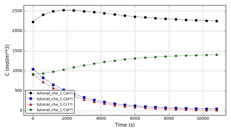
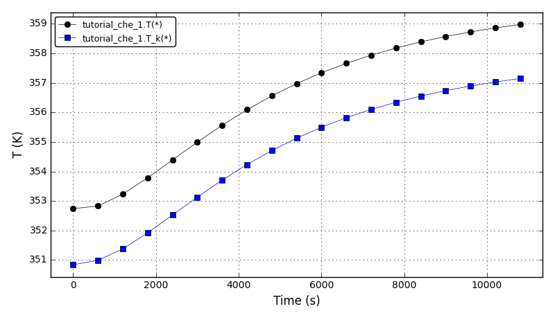
5.1. Chem. Eng. Example 1
Continuously Stirred Tank Reactor with energy balance and Van de Vusse reactions:
 A -> B -> C
2A -> D
Reference: G.A. Ridlehoover, R.C. Seagrave. Optimization of Van de Vusse Reaction Kinetics Using Semibatch Reactor Operation, Ind. Eng. Chem. Fundamen. 1973;12(4):444-447. doi:10.1021/i160048a700
The concentrations plot:
The temperatures plot:
Files
Model report |
|
Runtime model report |
|
Source code |
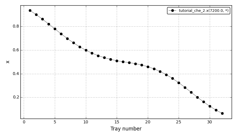
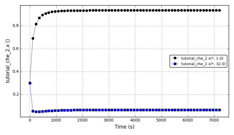
5.2. Chem. Eng. Example 2
Binary distillation column model.
Reference: J. Hahn, T.F. Edgar. An improved method for nonlinear model reduction using balancing of empirical gramians. Computers and Chemical Engineering 2002; 26:1379-1397. doi:10.1016/S0098-1354(02)00120-5
The liquid fraction after 120 min (x(reboiler)=0.935420, x(condenser)=0.064581):
The liquid fraction in the reboiler (tray 1) and in the condenser (tray 32):
Files
Model report |
|
Runtime model report |
|
Source code |
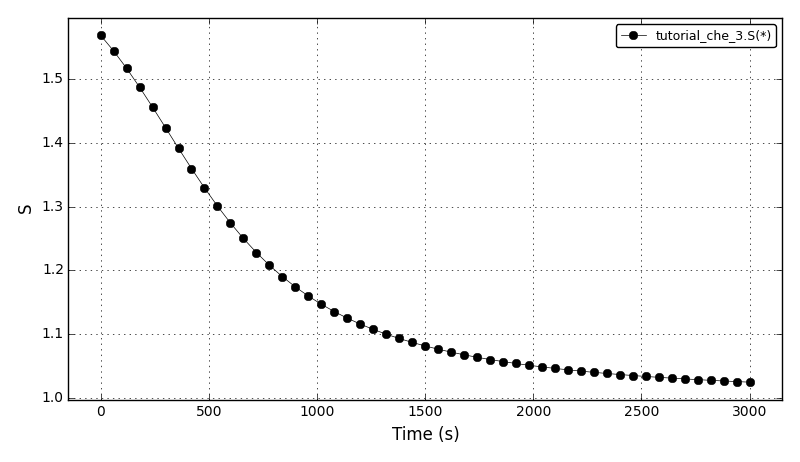
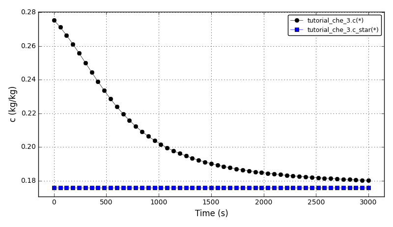
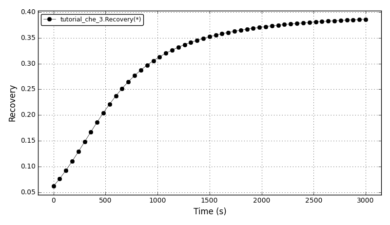
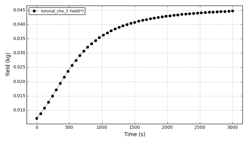
5.3. Chem. Eng. Example 3
Batch reactor seeded crystallisation using the method of moments.
References (model equations and input parameters):
Nikolic D.D., Frawley P.J. (2016) Application of the Lagrangian Meshfree Approach to Modelling of Batch Crystallisation: Part I - Modelling of Stirred Tank Hydrodynamics. Chemical Engineering Science 145:317-328. doi:10.1016/j.ces.2015.08.052
Mitchell N.A., O’Ciardha C.T., Frawley P.J. (2011) Estimation of the growth kinetics for the cooling crystallisation of paracetamol and ethanol solutions. Journal of Crystal Growth 328:39-49. doi:10.1016/j.jcrysgro.2011.06.016
The main assumptions:
Seeded crystallisation
Ideal mixing
Fixed cooling rate
Size independent growth
Solubility of Paracetamol in ethanol:
---------------------------------------------------------
Temperature       Solubility          Solubility
     C        kg Parac./kg EtOH   mol Parac./m3 EtOH
---------------------------------------------------------
      0           0.11362                593.0387
     10           0.14128                737.4215
     20           0.17568                916.9562
     30           0.21845                1140.2008
     40           0.27163                1417.7972
     50           0.33777                1762.9779
     60           0.42000                2192.1973
---------------------------------------------------------
The supersaturation plot:
The concentration plot:
The recovery plot:
The yield plot:
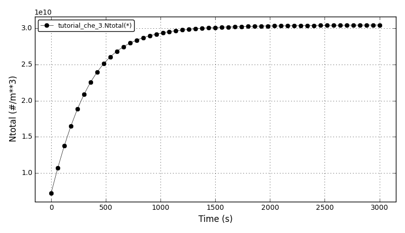
The total number of crystals plot:
Files
Model report |
|
Runtime model report |
|
Source code |
5.4. Chem. Eng. Example 4
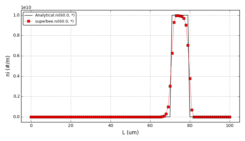
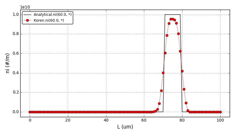
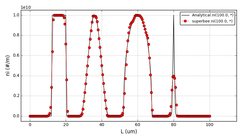
This example shows a comparison between the analytical results and the discretised population balance equations results solved using the cell centered finite volume method employing the high resolution upwind scheme (Van Leer k-interpolation with k = 1/3) and a range of flux limiters.
This tutorial can be run from the console only.
The problem is from the section 4.1.1 Size-independent growth I of the following article:
Nikolic D.D., Frawley P.J. Application of the Lagrangian Meshfree Approach to Modelling of Batch Crystallisation: Part II – An Efficient Solution of Integrated CFD and Population Balance Equations. Preprints 2016, 20161100128. doi:10.20944/preprints201611.0012.v1
and also from the section 3.1 Size-independent growth of the following article:
Qamar S., Elsner M.P., Angelov I.A., Warnecke G., Seidel-Morgenstern A. (2006) A comparative study of high resolution schemes for solving population balances in crystallization. Computers and Chemical Engineering 30(6-7):1119-1131. doi:10.1016/j.compchemeng.2006.02.012
The growth-only crystallisation process was considered with the constant growth rate of 1μm/s and the following initial number density function:
n(L,0): 1E10, if 10μm < L < 20μm
           0, otherwise
The crystal size in the range of [0, 100]μm was discretised into 100 elements. The analytical solution in this case is equal to the initial profile translated right in time by a distance Gt (the growth rate multiplied by the time elapsed in the process).
The flux limiters used in the model are:
HCUS
HQUICK
Koren
monotinized_central
minmod
Osher
ospre
smart
superbee
Sweby
UMIST
vanAlbada1
vanAlbada2
vanLeer
vanLeer_minmod
Comparison of L1- and L2-norms (ni_HR - ni_analytical):
--------------------------------------
         Scheme  L1         L2
--------------------------------------
       superbee  1.786e+10  7.016e+09
          Sweby  2.817e+10  8.614e+09
          Koren  3.015e+10  9.293e+09
          smart  2.961e+10  9.326e+09
             MC  3.258e+10  9.807e+09
           HCUS  3.638e+10  1.001e+10
         HQUICK  3.622e+10  1.005e+10
  vanLeerMinmod  3.581e+10  1.011e+10
        vanLeer  3.874e+10  1.059e+10
          ospre  4.139e+10  1.094e+10
          UMIST  4.363e+10  1.136e+10
          Osher  4.579e+10  1.156e+10
     vanAlbada1  4.574e+10  1.157e+10
         minmod  5.653e+10  1.325e+10
     vanAlbada2  5.456e+10  1.331e+10
 -------------------------------------
The comparison of number density functions between the analytical solution and the solution obtained using high-resolution scheme with the Superbee flux limiter at t=60s:
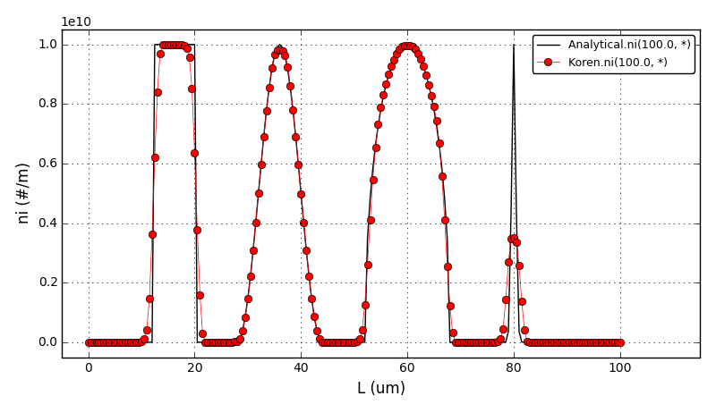
The comparison of number density functions between the analytical solution and the solution obtained using high-resolution scheme with the Koren flux limiter at t=60s:
Animation:
Files
Source code |
|
Analytical solution |
5.5. Chem. Eng. Example 5
Similar to the chem. eng. example 4, this example shows a comparison between the analytical results and the discretised population balance equations results solved using the cell centered finite volume method employing the high resolution upwind scheme (Van Leer k-interpolation with k = 1/3) and a range of flux limiters.
This tutorial can be run from the console only.
The problem is from the section 4.1.2 Size-independent growth II of the following article:
Nikolic D.D., Frawley P.J. Application of the Lagrangian Meshfree Approach to Modelling of Batch Crystallisation: Part II – An Efficient Solution of Integrated CFD and Population Balance Equations. Preprints 2016, 20161100128. doi:10.20944/preprints201611.0012.v1
and also from the section 3.2 Size-independent growth of the following article:
Qamar S., Elsner M.P., Angelov I.A., Warnecke G., Seidel-Morgenstern A. (2006) A comparative study of high resolution schemes for solving population balances in crystallization. Computers and Chemical Engineering 30(6-7):1119-1131. doi:10.1016/j.compchemeng.2006.02.012
Again, the growth-only crystallisation process was considered with the constant growth rate of 0.1μm/s and with the different initial number density function:
n(L,0):                      0, if        L <= 2.0μm
                          1E10, if  2μm < L <= 10μm (region I)
                             0, if 10μm < L <= 18μm
      1E10*cos^2(pi*(L-26)/64), if 18μm < L <= 34μm (region II)
                             0, if 34μm < L <= 42μm
      1E10*sqrt(1-(L-50)^2/64), if 42μm < L <= 58μm (region III)
                             0, if 58μm < L <= 66μm
1E10*exp(-(L-70)^2/(2sigma^2)), if 66μm < L <= 74μm (region IV)
                             0, if 74μm < L
The crystal size in the range of [0, 100]μm was discretised into 200 elements. The analytical solution in this case is equal to the initial profile translated right in time by a distance Gt (the growth rate multiplied by the time elapsed in the process).
Comparison of L1- and L2-norms (ni_HR - ni_analytical):
-------------------------------------
        Scheme  L1         L2
-------------------------------------
      superbee  4.464e+10  1.015e+10
         smart  4.727e+10  1.120e+10
         Koren  4.861e+10  1.141e+10
         Sweby  5.435e+10  1.142e+10
            MC  5.129e+10  1.162e+10
        HQUICK  5.531e+10  1.194e+10
          HCUS  5.528e+10  1.194e+10
 vanLeerMinmod  5.600e+10  1.202e+10
       vanLeer  5.814e+10  1.225e+10
         ospre  6.131e+10  1.252e+10
         UMIST  6.181e+10  1.259e+10
         Osher  6.690e+10  1.275e+10
    vanAlbada1  6.600e+10  1.281e+10
        minmod  7.751e+10  1.360e+10
    vanAlbada2  7.901e+10  1.413e+10
-------------------------------------
The comparison of number density functions between the analytical solution and the solution obtained using high-resolution scheme with the Superbee flux limiter at t=100s:
The comparison of number density functions between the analytical solution and the solution obtained using high-resolution scheme with the Koren flux limiter at t=100s:
Files
Source code |
|
Analytical solution |
5.6. Chem. Eng. Example 6
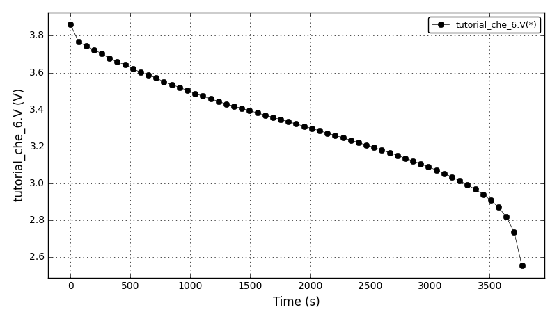
Model of a lithium-ion battery based on porous electrode theory as developed by John Newman and coworkers. In particular, the equations here are based on a summary of the methodology by Karen E. Thomas, John Newman, and Robert M. Darling,
Thomas K., Newman J., Darling R. (2002). Mathematical Modeling of Lithium Batteries in Advances in Lithium-ion Batteries. Springer US. 345-392. doi:10.1007/0-306-47508-1_13
A few simplifications have been made rather than implementing the more complete model described there. For example, the following assumptions have (currently) been made:
two porous electrodes are used rather than providing the option for a “half cell” in which one electrode is lithium foil.
conductivity in the electron-conducting phase is infinite
constant exchange current density in Butler-Volmer reaction expression
no electrolyte convection
constant and uniform solvent concentration (ions vary according to concentrated solution theory)
monodisperse particles in electrode
no volume occupied by binder, filler, etc. in the electrode
The up to date version of the model is available at Raymond’s GitHub repository: https://github.com/raybsmith/daetools-example-battery.
The voltage plot:
The current plot:

Files
Model report |
|
Runtime model report |
|
Source code |
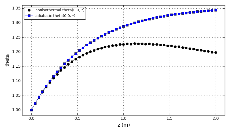
5.7. Chem. Eng. Example 7
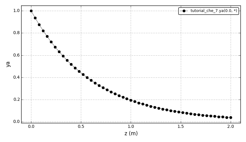
Steady-state Plug Flow Reactor with energy balance and first order reaction:
A -> B
The problem is example 9.4.3 from the section 9.4 Nonisothermal Plug Flow Reactor from the following book:
Davis M.E., Davis R.J. (2003) Fundamentals of Chemical Reaction Engineering. McGraw Hill, New York, US. ISBN 007245007X.
The dimensionless concentration plot:
The dimensionless temperature plot (adiabatic and nonisothermal cases):
Files
Model report |
|
Runtime model report |
|
Source code |
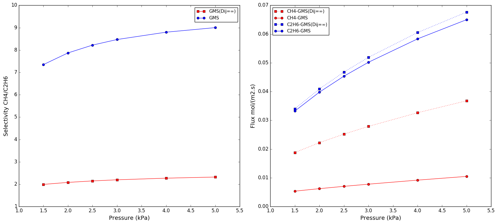
5.8. Chem. Eng. Example 8
Model of a gas separation on a porous membrane with a metal support. The model employs the Generalised Maxwell-Stefan (GMS) equations to predict fluxes and selectivities. The membrane unit model represents a generic two-dimensonal model of a porous membrane and consists of four models:
Retentate compartment (isothermal axially dispersed plug flow)
Micro-porous membrane
Macro-porous support layer
Permeate compartment (the same transport phenomena as in the retentate compartment)
The retentate compartment, the porous membrane, the support layer and the permeate compartment are coupled via molar flux, temperature, pressure and gas composition at the interfaces. The model is described in the section 2.2 Membrane modelling of the following article:
Nikolic D.D., Kikkinides E.S. (2015) Modelling and optimization of PSA/Membrane separation processes. Adsorption 21(4):283-305. doi:10.1007/s10450-015-9670-z
and in the original Krishna article:
Krishna R. (1993) A unified approach to the modeling of intraparticle diffusion in adsorption processes. Gas Sep. Purif. 7(2):91-104. doi:10.1016/0950-4214(93)85006-H
This version is somewhat simplified for it only offers an extended Langmuir isotherm. The Ideal Adsorption Solution theory (IAS) and the Real Adsorption Solution theory (RAS) described in the articles are not implemented here.
The problem modelled is separation of hydrocarbons (CH4+C2H6) mixture on a zeolite (silicalite-1) membrane with a metal support from the section ‘Binary mixture permeation’ of the following article:
van de Graaf J.M., Kapteijn F., Moulijn J.A. (1999) Modeling Permeation of Binary Mixtures Through Zeolite Membranes. AIChE J. 45:497–511. doi:10.1002/aic.690450307
The CH4 and C2H6 fluxes, and CH4/C2H6 selectivity plots for two cases: GMS and GMS(Dij=∞), 1:1 mixture, and T = 303 K:
Files
Model report |
|
Runtime model report |
|
Source code |
|
Membrane unit |
|
Variable types |
|
Membrane model |
|
Support model |
|
In/out compartment |
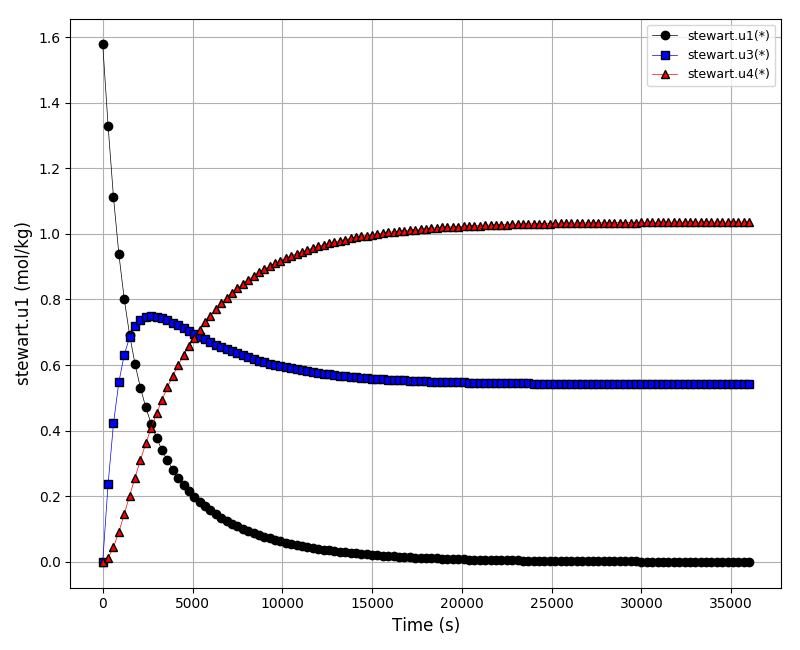
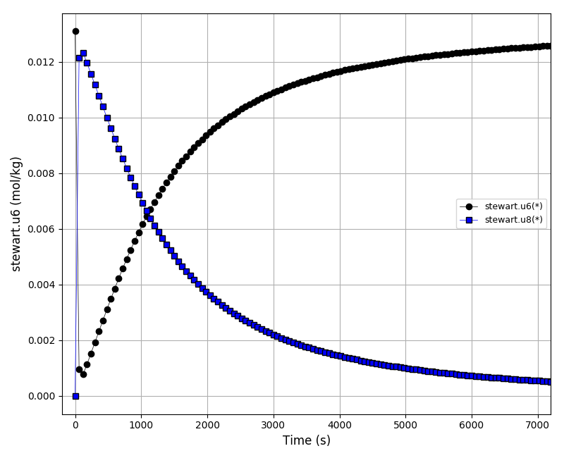
5.9. Chem. Eng. Example 9
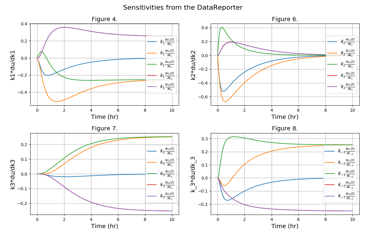
Chemical reaction network from the Dow Chemical Company described in the following article:
Caracotsios M., Stewart W.E. (1985) Sensitivity analysis of initial value problems with mixed odes and algebraic equations. Computers & Chemical Engineering 9(4):359-365. doi:10.1016/0098-1354(85)85014-6
The sensitivity analysis is enabled and the sensitivity data can be obtained in two ways:
Directly from the DAE solver in the user-defined Run function using the DAESolver.SensitivityMatrix property.
From the data reporter as any ordinary variable.
The concentrations plot (u1, u3, u4):
The concentrations plot (u6, u8):
The sensitivities plot (k2*du1/dk2, k2*du2/dk2, k2*du3/dk2, k2*du4/dk2, k2*du5/dk2):
Files
Model report |
|
Runtime model report |
|
Source code |