3. Code Verification Tests
Code verification method using the Method of Exact Solutions (sensitivity analysis; first order differential equations with constant coefficients). |
|
Code verification method using the Method of Manufactured Solutions (1D transient convection-diffusion equation with Dirichlet boundary conditions). |
|
Code verification method using the Method of Manufactured Solutions (1D transient convection-diffusion equation with Neumann boundary conditions). |
|
Code verification method using the Method of Manufactured Solutions (2D transient convection-diffusion equation with Dirichlet boundary conditions). |
|
Code verification method using the Method of Manufactured Solutions (1D transient conduction equation using the Finite Elements method). |
|
Code verification method using the Method of Exact Solutions (1D homogeneous transient convection-diffusion equation solved using the high-resolution upwind finite volume scheme with flux limiter). |
|
Code verification method using the Method of Manufactured Solutions (1D steady-state convection-diffusion-reaction equation solved using the high-resolution upwind finite volume scheme with flux limiter). |
|
Code verification method using the Method of Manufactured Solutions (1D transient convection-diffusion-reaction equation solved using the high-resolution upwind finite volume scheme with flux limiter). |
|
Code verification using the Method of Exact Solutions (Solid Body Rotation problem solved using the Finite Elements method). |
|
Code verification using the Method of Exact Solutions (Rotating Gaussian Hill problem solved using the Finite Elements method). |
|
Code verification method using the Method of Exact Solutions (1D homogeneous transient convection-diffusion equation solved using the high-resolution upwind finite volume scheme with flux limiter for the reversed fluid flow). |
3.1. Code Verification Test 1
Code verification using the Method of Exact Solutions.
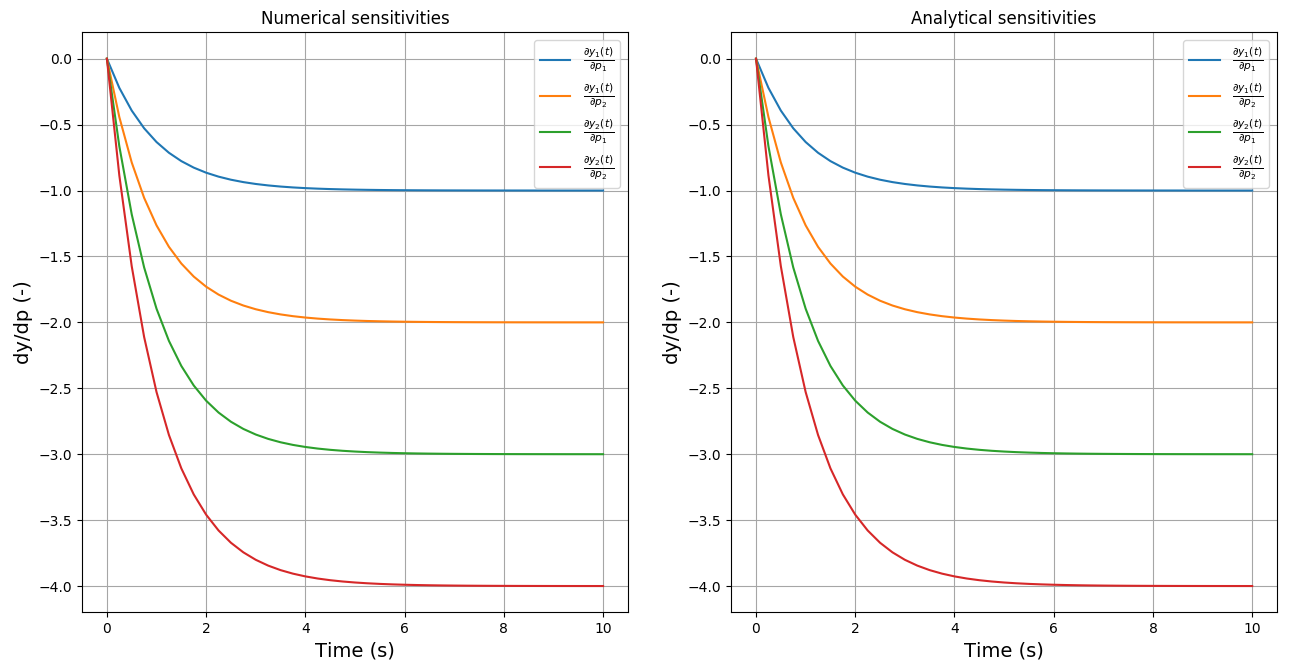
Here, the numerical solution and numerical sensitivities for the Constant coefficient first order equations are compared to the available analytical solution.
The sensitivity analysis is enabled and the sensitivities are reported to the data reporter. The sensitivity data can be obtained in two ways:
Directly from the DAE solver in the user-defined Run function using the DAESolver.SensitivityMatrix property.
From the data reporter as any ordinary variable.
The comparison between the numerical and the analytical sensitivities:
Files
Model report |
|
Runtime model report |
|
Source code |
3.2. Code Verification Test 2
Code verification using the Method of Manufactured Solutions.
References:
G. Tryggvason. Method of Manufactured Solutions, Lecture 33: Predictivity-I, 2011. PDF
K. Salari and P. Knupp. Code Verification by the Method of Manufactured Solutions. SAND2000 – 1444 (2000). doi:10.2172/759450
P.J. Roache. Fundamentals of Verification and Validation. Hermosa, 2009. ISBN-10:0913478121
The procedure for the transient convection-diffusion (Burger’s) equation:
L(f) = df/dt + f*df/dx - D*d2f/dx2 = 0
is the following:
Pick a function (q, the manufactured solution):
q = A + sin(x + Ct)
Compute the new source term (g) for the original problem:
g = dq/dt + q*dq/dx - D*d2q/dx2
Solve the original problem with the new source term:
df/dt + f*df/dx - D*d2f/dx2 = g
Since L(f) = g and g = L(q), consequently we have: f = q. Therefore, the computed numerical solution (f) should be equal to the manufactured one (q).
The terms in the source g term are:
dq/dt   = C * cos(x + C*t)
dq/dx   = cos(x + C*t)
d2q/dx2 = -sin(x + C*t)
The equations are solved for Dirichlet boundary conditions:
f(x=0)   = q(x=0)   = A + sin(0 + Ct)
f(x=2pi) = q(x=2pi) = A + sin(2pi + Ct)
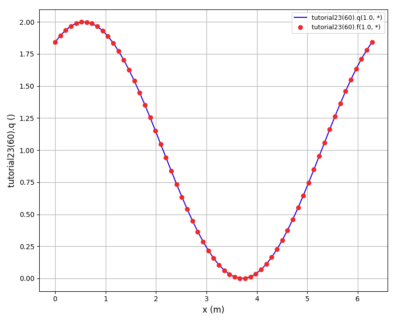
Numerical vs. manufactured solution plot (no. elements = 60, t = 1.0s):
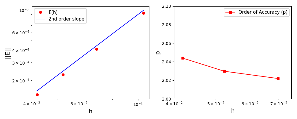
The normalised global errors and the order of accuracy plots (no. elements = [60, 90, 120, 150], t = 1.0s):
Files
Model report |
|
Runtime model report |
|
Source code |
3.3. Code Verification Test 3
Code verification using the Method of Manufactured Solutions.
References:
G. Tryggvason. Method of Manufactured Solutions, Lecture 33: Predictivity-I, 2011. PDF
K. Salari and P. Knupp. Code Verification by the Method of Manufactured Solutions. SAND2000 – 1444 (2000). doi:10.2172/759450
P.J. Roache. Fundamentals of Verification and Validation. Hermosa, 2009. ISBN-10:0913478121
The problem in this tutorial is identical to tutorial_cv_3. The only difference is that the Neumann boundary conditions are applied:
df(x=0)/dx   = dq(x=0)/dx   = cos(0 + Ct)
df(x=2pi)/dx = dq(x=2pi)/dx = cos(2pi + Ct)
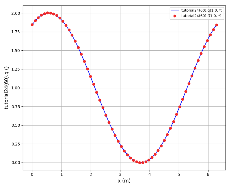
Numerical vs. manufactured solution plot (no. elements = 60, t = 1.0s):
The normalised global errors and the order of accuracy plots (no. elements = [60, 90, 120, 150], t = 1.0s):
Files
Model report |
|
Runtime model report |
|
Source code |
3.4. Code Verification Test 4
Code verification using the Method of Manufactured Solutions.
Reference:
K. Salari and P. Knupp. Code Verification by the Method of Manufactured Solutions. SAND2000 – 1444 (2000). doi:10.2172/759450
The problem in this tutorial is the transient convection-diffusion equation distributed on a rectangular 2D domain with u and v components of velocity:
L(u) = du/dt + (d(uu)/dx + d(uv)/dy) - ni * (d2u/dx2 + d2u/dy2) = 0
L(v) = dv/dt + (d(vu)/dx + d(vv)/dy) - ni * (d2v/dx2 + d2v/dy2) = 0
The manufactured solutions are:
um = u0 * (sin(x**2 + y**2 + w0*t) + eps)
vm = v0 * (cos(x**2 + y**2 + w0*t) + eps)
The terms in the new sources Su and Sv are computed using the daetools derivative functions (dt, d and d2).
Again, the Dirichlet boundary conditions are used:
u(LB, y)  = um(LB, y)
u(UB, y)  = um(UB, y)
u(x,  LB) = um(x,  LB)
u(x,  UB) = um(x,  UB)

v(LB, y)  = vm(LB, y)
v(UB, y)  = vm(UB, y)
v(x,  LB) = vm(x,  LB)
v(x,  UB) = vm(x,  UB)
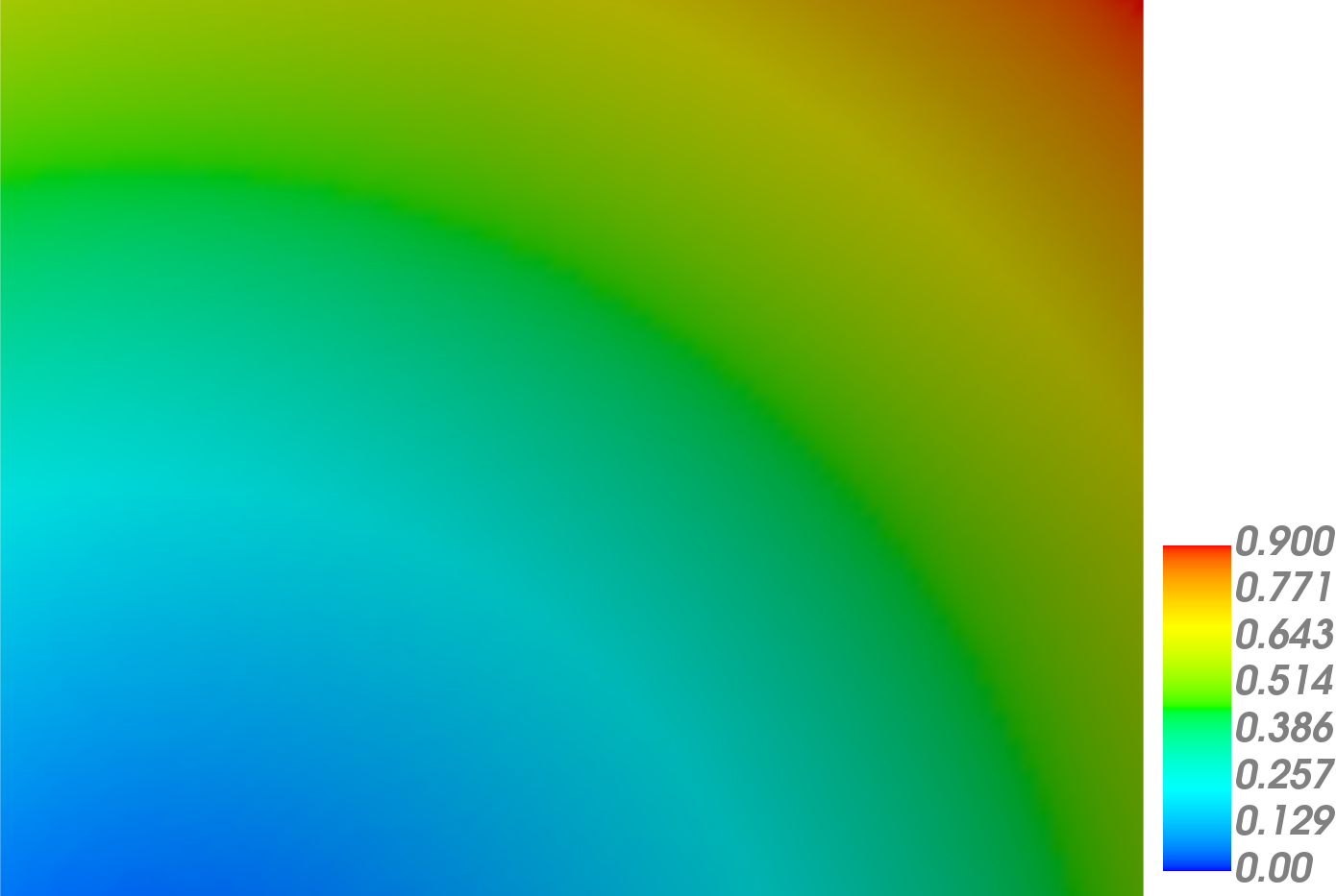
Steady-state results (w0 = 0.0) for the u-component:
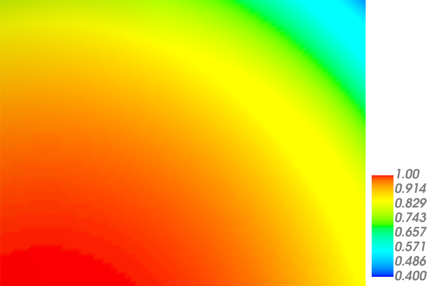
Steady-state results (w0 = 0.0) for the v-component:
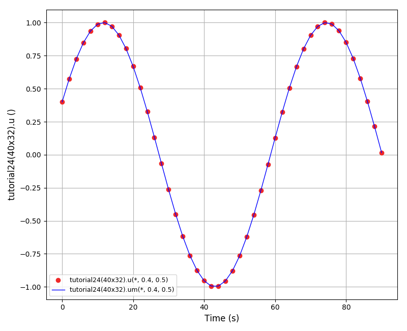
Numerical vs. manufactured solution plot (u velocity component, 40x32 grid):
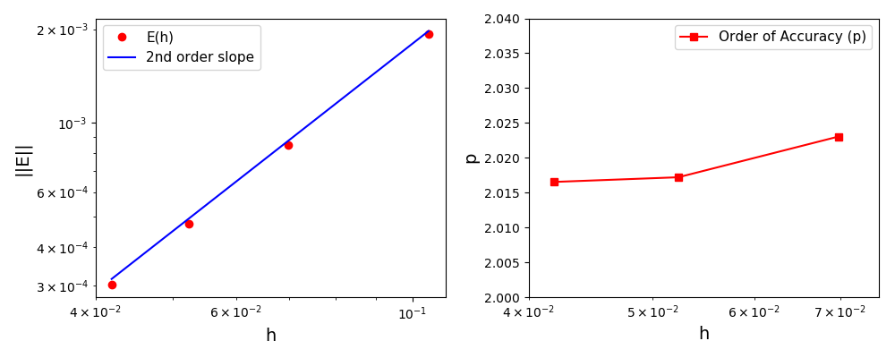
The normalised global errors and the order of accuracy plots (grids 10x8, 20x16, 40x32, 80x64):
Files
Model report |
|
Runtime model report |
|
Source code |
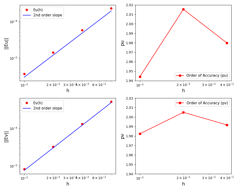
3.5. Code Verification Test 5
Code verification using the Method of Manufactured Solutions.
This problem and its solution in COMSOL Multiphysics software is described in the COMSOL blog: Verify Simulations with the Method of Manufactured Solutions (2015).
Here, a 1D transient heat conduction problem in a bar of length L is solved using the FE method:
dT/dt - k/(rho*cp) * d2T/dx2 = 0, x in [0,L]
with the following boundary:
T(0,t) = 500 K
T(L,t) = 500 K
and initial conditions:
T(x,0) = 500 K
The manufactured solution is given by function u(x):
u(x) = 500 + (x/L) * (x/L - 1) * (t/tau)
The new source term is:
g(x) = du/dt - k/(rho*cp) * d2u/dx2
The terms in the source g term are:
du_dt   = (x/L) * (x/L - 1) * (1/tau)
d2u_dx2 = (2/(L**2)) * (t/tau)
Finally, the original problem with the new source term is:
dT/dt - k/(rho*cp) * d2T/dx2 = g(x), x in [0,L]
The mesh is linear (a bar) with a length of 100 m:
-20.png)
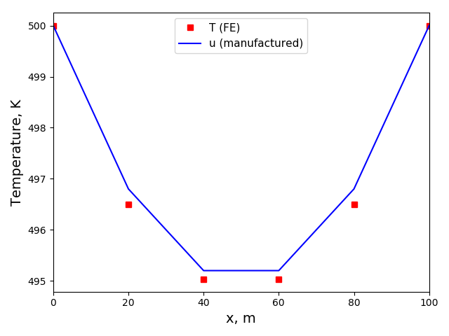
The comparison plots for the coarse mesh and linear elements:
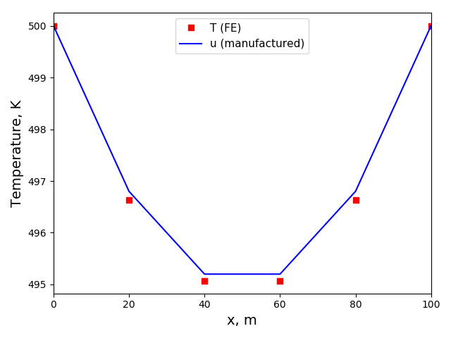
The comparison plots for the coarse mesh and quadratic elements:
The comparison plots for the fine mesh and linear elements:
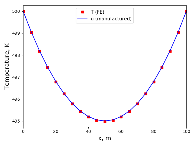
The comparison plots for the fine mesh and quadratic elements:

Files
Model report |
|
Runtime model report |
|
Source code |
3.6. Code Verification Test 6
Code verification using the Method of Exact Solutions.
Reference (section 3.3):
B. Koren. A robust upwind discretization method for advection, diffusion and source terms. Department of Numerical Mathematics. Report NM-R9308 (1993). PDF
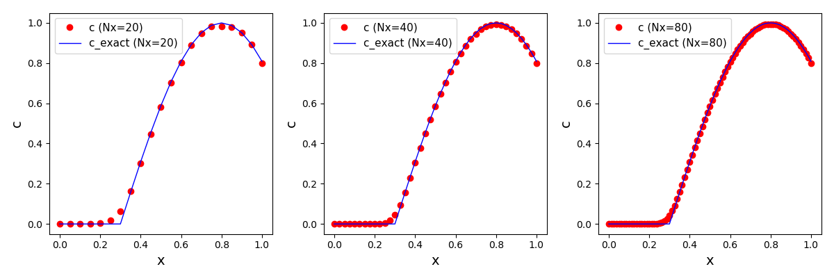
The problem in this tutorial is 1D transient convection-diffusion equation:
dc_dt + u*dc/dx - D*d2c/dc2 = 0
The equation is solved using the high resolution cell-centered finite volume upwind scheme with flux limiter described in the article.
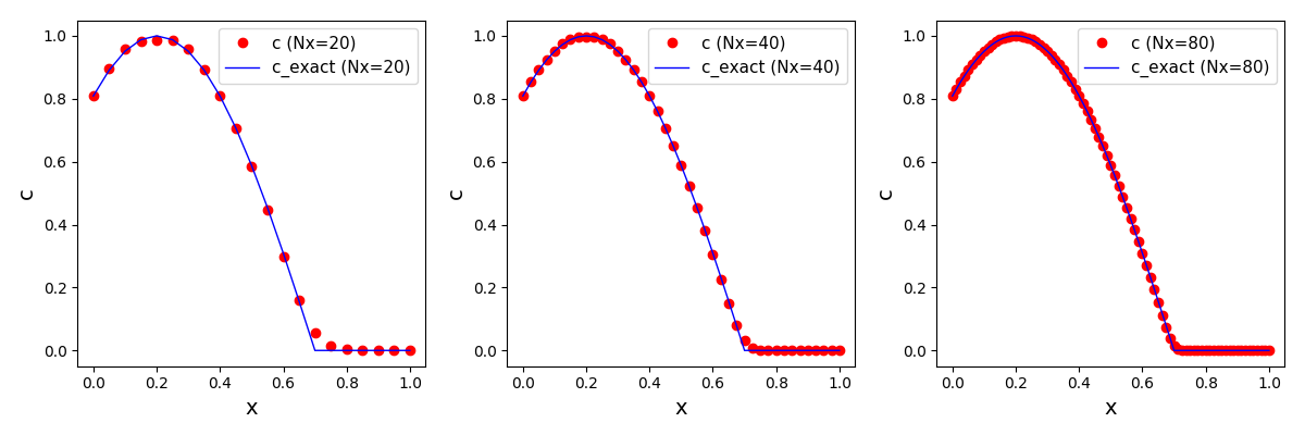
Numerical vs. exact solution plots (Nx = [20, 40, 80]):
Files
Model report |
|
Runtime model report |
|
Source code |
3.7. Code Verification Test 7
Code verification using the Method of Manufactured Solutions.
Reference (section 4.2):
B. Koren. A robust upwind discretization method for advection, diffusion and source terms. Department of Numerical Mathematics. Report NM-R9308 (1993). PDF
The problem in this tutorial is 1D steady-state convection-diffusion (Burger’s) equation:
u*dc/dx - D*d2c/dc2 = 0
The manufactured solution is:
c(x) = 0.5 * (1 - cos(2*pi*(x-a)/(b-a))), x in [a,b]
c(x) = 0, otherwise
The new source term is:
s(x) = pi/(b-a) * u * sin(2*pi*(x-a)/(b-a)) - 2*(pi/(b-a))**2 * D * cos(2*pi*(x-a)/(b-a)), x in [a,b]
s(x) = 0, otherwise
The modified equation:
u*dc/dx - D*d2c/dc2 = s(x)
is solved using the high resolution cell-centered finite volume upwind scheme with flux limiter described in the article.
In order to obtain the consistent discretisation of the convection and the source terms an integral of the source term: S(x) = 1/u * Integral s(x)*dx must be calculated. The result of integration is given as:
S(x) = 0.5 * (1 - cos(2*pi*(x-a)/(b-a)))) - pi/(b-a) * D/u * sin(2*pi*(x-a)/(b-a))), x in [a,b]
S(x) = 0, otherwise
Numerical vs. manufactured solution plot (Nx=80):
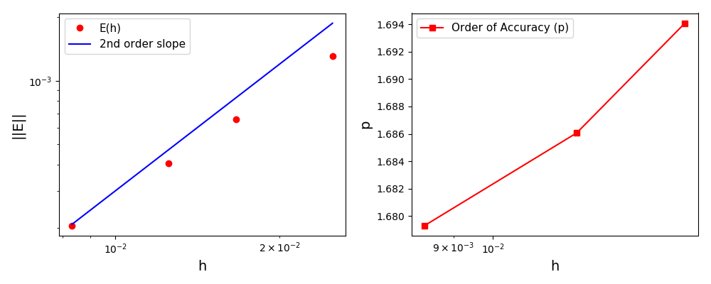
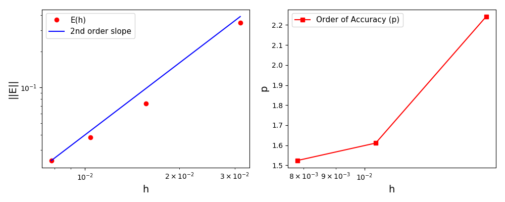
The normalised global errors and the order of accuracy plots for the Koren flux limiter (grids 40, 60, 80, 120):
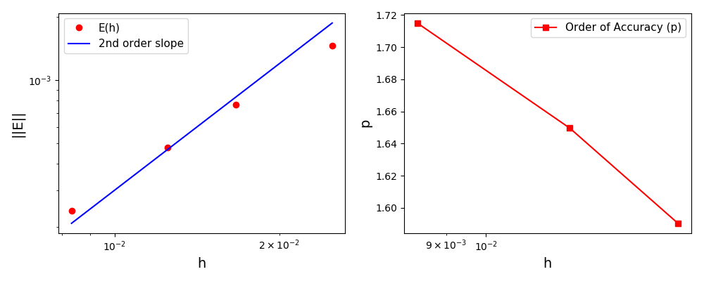
The normalised global errors and the order of accuracy plots for the Superbee flux limiter (grids 40, 60, 80, 120):
Files
Model report |
|
Runtime model report |
|
Source code |
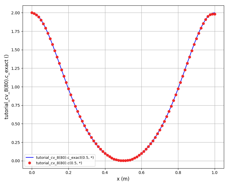
3.8. Code Verification Test 8
Code verification using the Method of Manufactured Solutions.
Reference (page 64):
W. Hundsdorfer. Numerical Solution of Advection-Diffusion-Reaction Equations. Lecture notes (2000), Thomas Stieltjes Institute. PDF
The problem in this tutorial is 1D transient convection-reaction equation:
dc/dt + dc/dx = c**2
The exact solution is:
c(x,t) = sin(pi*(x-t))**2 / (1 - t*sin(pi*(x-t))**2)
The equation is solved using the high resolution cell-centered finite volume upwind scheme with flux limiter described in the article. The boundary and initial conditions are obtained from the exact solution.
The consistent discretisation of the convection and the source terms cannot be done since the constant C1 in the integral of the source term:
S(x) = 1/u * Integral s(x)*dx = u**/3 + C1
is not known. Therefore, the numerical cell average is used:
Snum(x) = Integral s(x)*dx = s(i) * (x[i]-x[i-1]).
Numerical vs. manufactured solution plot (Nx=80):
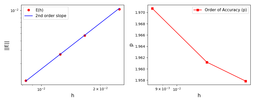
The normalised global errors and the order of accuracy plots for the Koren flux limiter (grids 40, 60, 80, 120):
Files
Model report |
|
Runtime model report |
|
Source code |
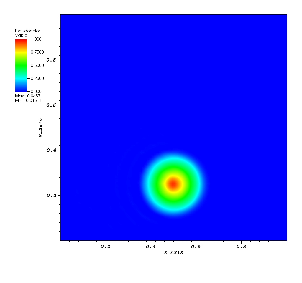
3.9. Code Verification Test 9
Code verification using the Method of Exact Solutions (Solid Body Rotation problem).
Reference (section 4.4.6.1 Solid Body Rotation):
D. Kuzmin (2010). A Guide to Numerical Methods for Transport Equations. PDF
Solid body rotation illustrates the ability of a numerical scheme to transport initial data without distortion. Here, a 2D transient convection problem in a rectangular (0,1)x(0,1) domain is solved using the FE method:
dc/dt + div(u*c) = 0, in Omega = (0,1)x(0,1)
The initial conditions define a conical body which is rotated counterclockwise around the point (0.5, 0.5) using the velocity field u = (0.5 - y, x - 0.5). The cone is defined by the following equation:
r0 = 0.15
(x0, y0) = (0.5, 0.25)
c(x,y,0) = 1 - (1/r0) * sqrt((x-x0)**2 + (y-y0)**2)
After t = 2pi the body should arrive at the starting position.
Homogeneous Dirichlet boundary conditions are prescribed at all four edges:
c(x,y,t) = 0.0
The mesh is a square (0,1)x(0,1):
x(0,1)-64x64.png)
The solution plot at t = 0 and t = 2pi (96x96 grid):

Animations for 32x32 and 96x96 grids:
It can be observed that the shape of the cone is preserved. Also, since the above equation is hyperbolic some oscillations in the solution out of the cone appear, which are more pronounced for coarser grids. This problem was resolved in the original example using the flux linearisation technique.
The normalised global errors and the order of accuracy plots (no. elements = [32x32, 64x64, 96x96, 128x128], t = 2pi):
Files
Model report |
|
Runtime model report |
|
Source code |
3.10. Code Verification Test 10
Code verification using the Method of Exact Solutions (Rotating Gaussian Hill problem).
Reference (section 4.4.6.3 Convection-Diffusion):
D. Kuzmin (2010). A Guide to Numerical Methods for Transport Equations. PDF
Here, a 2D transient convection-diffusion problem in a rectangular (-1,1)x(-1,1) domain is solved using the FE method:
dc/dt + div(u*c) - eps*nabla(c) = 0, in Omega = (-1,1)x(-1,1)
The exact solution is given by the following function:
(x0, y0) = (0.0, 0.5)
x_bar(t) = x0*cos(t) - y0*sin(t)
y_bar(t) = -x0*sin(t) + y0*cos(t)
r2(x,y,t) = (x-x_bar(t))**2 + (y-y_bar(t))**2

c_exact(x,y,t) = 1.0 / (4*pi*eps*t) * exp(-r2(x,y,t) / (4*eps*t))
The initial conditions define a Gaussian hill which is rotated counterclockwise around the point (0.0, 0.0) using the velocity field u = (-y, x). Since at t = 0 the value of c_exact is the Dirac delta function it is better to start the simulation at t > 0. Therefore, the simulation is started and t = pi/2 by reinitialising variable c to:
c(x,y,pi/2) = c_exact(x,y,pi/2)
At t = 5/2 pi the peak smeared by the diffusion should arrive at the starting position.
Homogeneous Dirichlet boundary conditions are prescribed at all four edges:
c(x,y,t) = 0.0
The mesh is a rectangle (-1,1)x(-1,1):
x(-1,1)-64x64.png)
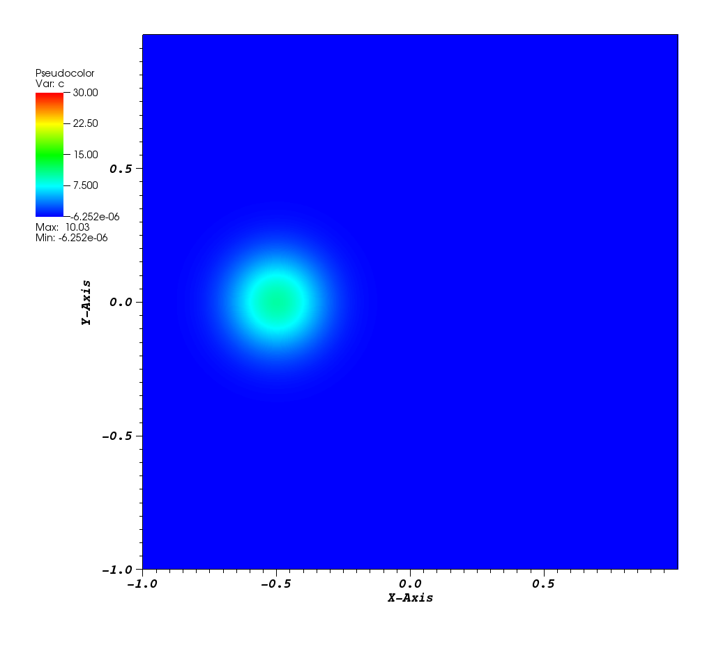
The solution plots at t = pi/2 (the initial peak) and t = 5/2pi (96x96 grid):

Animations for 32x32 and 96x96 grids:
Again, some low-magnitude oscillations in the solution appear, which are more pronounced for coarser grids. In the original example this problem was resolved using the flux linearisation technique.
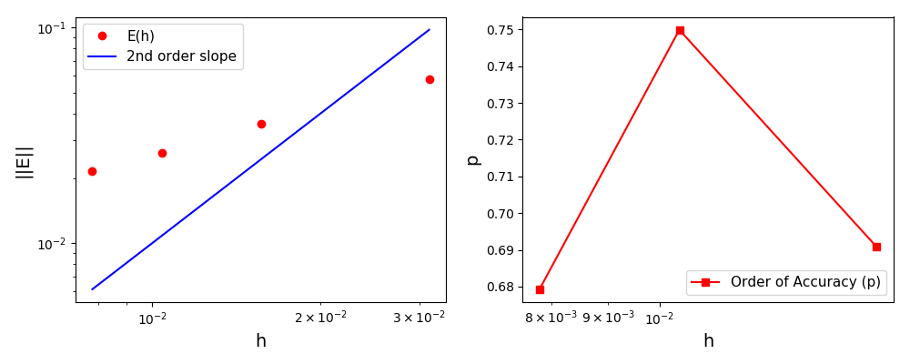
The normalised global errors and the order of accuracy plots (no. elements = [32x32, 64x64, 96x96, 128x128], t = 5/2pi):
Files
Model report |
|
Runtime model report |
|
Source code |
3.11. Code Verification Test 11
Code verification using the Method of Exact Solutions.
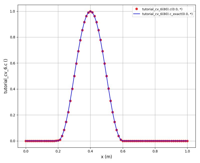
The problem is identical to the problem in the tutorial_cv_6. The only difference is that the flow is reversed to test the high resolution scheme for the reversed flow mode.
Numerical vs. exact solution plots (Nx = [20, 40, 80]):
Files
Model report |
|
Runtime model report |
|
Source code |