2. Advanced Tutorials
Interactive operating procedures (pyQt GUI). |
|
Solution of a discretized population balance using high resolution upwind schemes with flux limiter. |
|
Using code-generators (Scilab/GNU_Octave/Matlab MEX functions, Simulink S-functions, Modelica/gPROMS/FMI code-generators). |
|
OpenCS code generator. |
2.1. Advanced Tutorial 1
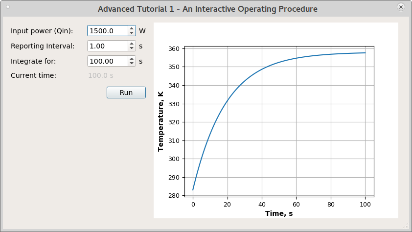
This tutorial presents a user-defined simulation which instead of simply integrating the system shows the pyQt graphical user interface (GUI) where the simulation can be manipulated (a sort of interactive operating procedure).
The model in this example is the same as in the tutorial 4.
The simulation.Run() function is modifed to show the graphical user interface (GUI) that allows to specify the input power of the heater (degree of freedom), a time period for integration, and a reporting interval. The GUI also contains the temperature plot updated in real time, as the simulation progresses.
The screenshot of the pyQt GUI:
Files
Model report |
|
Runtime model report |
|
Source code |
2.2. Advanced Tutorial 2
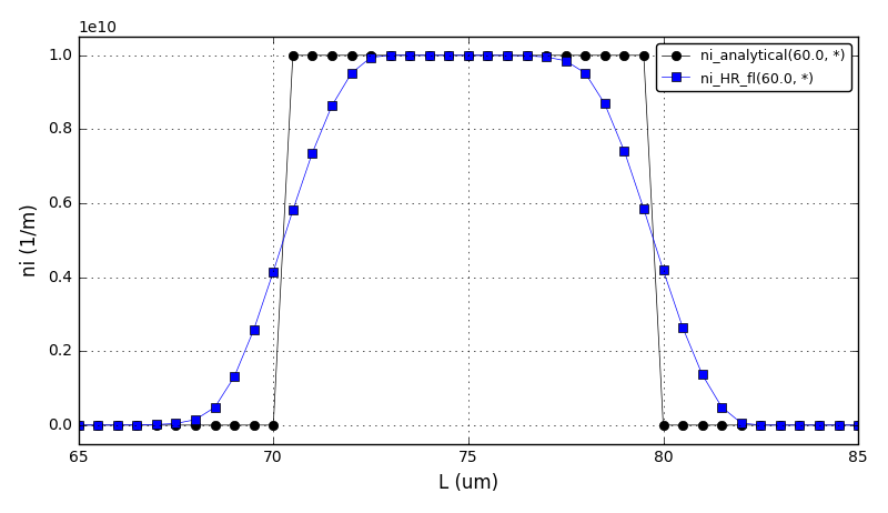
This tutorial demonstrates a solution of a discretized population balance using high resolution upwind schemes with flux limiter.
Reference: Qamar S., Elsner M.P., Angelov I.A., Warnecke G., Seidel-Morgenstern A. (2006) A comparative study of high resolution schemes for solving population balances in crystallization. Computers and Chemical Engineering 30(6-7):1119-1131. doi:10.1016/j.compchemeng.2006.02.012
It shows a comparison between the analytical results and various discretization schemes:
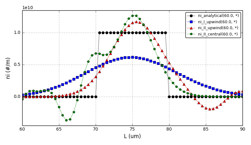
I order upwind scheme
II order central scheme
Cell centered finite volume method solved using the high resolution upwind scheme (Van Leer k-interpolation with k = 1/3 and Koren flux limiter)
The problem is from the section 3.1 Size-independent growth.
Could be also found in: Motz S., Mitrović A., Gilles E.-D. (2002) Comparison of numerical methods for the simulation of dispersed phase systems. Chemical Engineering Science 57(20):4329-4344. doi:10.1016/S0009-2509(02)00349-4
The comparison of number density functions between the analytical solution and the high-resolution scheme:
The comparison of number density functions between the analytical solution and the I order upwind, II order upwind and II order central difference schemes:
Files
Model report |
|
Runtime model report |
|
Source code |
2.3. Advanced Tutorial 3
This tutorial introduces the following concepts:
DAE Tools code-generators
Modelica code-generator
gPROMS code-generator
FMI code-generator (for Co-Simulation)
DAE Tools model-exchange capabilities:
Scilab/GNU_Octave/Matlab MEX functions
Simulink S-functions
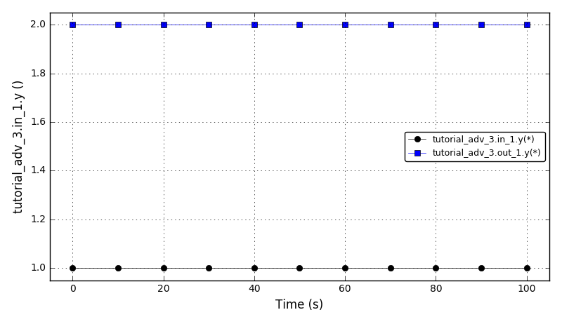
The model represent a simple multiplier block. It contains two inlet and two outlet ports. The outlets values are equal to inputs values multiplied by a multiplier “m”:
out1.y   = m1   x in1.y
out2.y[] = m2[] x in2.y[]
where multipliers m1 and m2[] are:
STN Multipliers
   case variableMultipliers:
      dm1/dt   = p1
      dm2[]/dt = p2
   case constantMultipliers:
      dm1/dt   = 0
      dm2[]/dt = 0
(that is the multipliers can be constant or variable).
The ports in1 and out1 are scalar (width = 1). The ports in2 and out2 are vectors (width = 1).
Achtung, Achtung!! Notate bene:
Inlet ports must be DOFs (that is to have their values asssigned), for they can’t be connected when the model is simulated outside of daetools context.
Only scalar output ports are supported at the moment!! (Simulink issue)
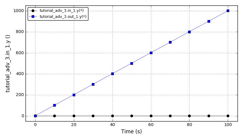
The plot of the inlet ‘y’ variable and the multiplied outlet ‘y’ variable for the constant multipliers (m1 = 2):
The plot of the inlet ‘y’ variable and the multiplied outlet ‘y’ variable for the variable multipliers (dm1/dt = 10, m1(t=0) = 2):
Files
Model report |
|
Runtime model report |
|
Source code |
2.4. Advanced Tutorial 4
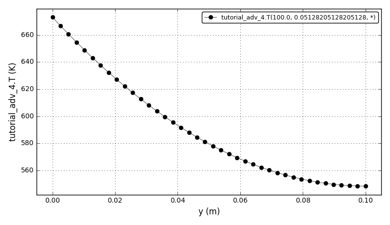
This tutorial illustrates the OpenCS code generator. For the given DAE Tools simulation it generates input files for OpenCS simulation, either for a single CPU or for a parallel simulation using MPI. The model is identical to the model in the tutorial 11.
The OpenCS framework currently does not support:
Discontinuous equations (STNs and IFs)
External functions
Thermo-physical property packages
The temperature plot (at t=100s, x=0.5128, y=*):
Files
Model report |
|
Runtime model report |
|
Source code |