1. Basic Tutorials
The key modelling concepts in DAE Tools:
Importing DAE Tools pyDAE module(s), units and variable types developing models, setting up a simulation, declaring auxiliary objects (DAE solver, data reporter, log), simulation run-time options, running a smulation. |
|
Using distribution domains, distributing parameters/variables/equations on domains, using derivative functions (dt, d, d2), setting boundary and initial conditions. |
|
Using arrays (discrete distribution domains), specifying degrees of freedom, setting initial guesses. |
|
Declaring arrays of variable values (Array function) and using functions that operate on them arrays, using the Constant function, making non-uniform grids. |
|
Using ports, making port connections, declaring components (instances of other models). |
|
Saving and restoring initialisation files, evaluating integrals. |
Support for discrete systems:
Declaring discontinuous equations (symmetrical state transition networks: daeIF statements). |
|
Declaring discontinuous equations (non-symmetrical state transition networks: daeSTN statements). |
|
Using event ports, handling events using ON_CONDITION() and ON_EVENT() functions, and declaring user defined actions. |
|
Declaring nested state transitions. |
The simulation options:
Making user-defined schedules (operating procedures), resetting the values of degrees of freedom and resetting initial conditions. |
Data reporting:
Using data reporters to write the results into files (Matlab, MS Excel, JSON, XML, HDF5, VTK, Pandas), developing custom data reporters. |
DAE and LA solvers:
Using available linear equations solvers (SuperLU, SuperLU_MT, Trilinos Amesos, IntelPardiso, Pardiso). |
|
Using iterative linear equations solvers (Trilinos AztecOO) and preconditioners (built-in AztecOO, Ifpack, ML). |
|
Using SuperLU and SuperLU_MT solvers and their options. |
External functions:
Declaring and using external functions. |
Logging:
Using TCPIP Log and TCPIPLogServer. |
Interoperability with NumPy:
Using DAE Tools variables and NumPy functions to solve a simple stationary 1D heat conduction by manually assembling Finite Element stiffness matrix and load vector. |
|
Using DAE Tools variables and NumPy functions to generate and solve a simple ODE system. |
Thermophysical property packages:
Using thermophysical property packages in DAE Tools. |
Variable constraints:
Specifying variable constraints in DAE Tools. |
Equation evaluation modes:
Specifying different equation evaluation modes and evaluators. |
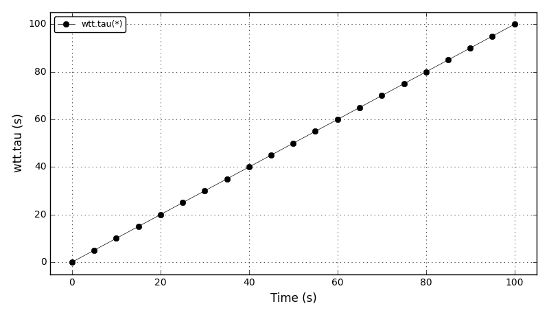
1.1. What’s the time? (AKA: Hello world!)
What is the time? (AKA Hello world!) is a very simple model. The model consists of a single variable (called ‘time’) and a single differential equation:
d(time)/dt = 1
This way, the value of the variable ‘time’ is equal to the elapsed time in the simulation.
This tutorial presents the basic structure of daeModel and daeSimulation classes. A typical DAETools simulation requires the following 8 tasks:
Importing DAE Tools pyDAE module(s)
Importing or declaration of units and variable types (unit and daeVariableType classes)
Developing a model by deriving a class from the base daeModel class and:
Declaring domains, parameters and variables in the daeModel.__init__ function
Declaring equations and their residual expressions in the daeModel.DeclareEquations function
Setting up a simulation by deriving a class from the base daeSimulation class and:
Specifying a model to be used in the simulation in the daeSimulation.__init__ function
Setting the values of parameters in the daeSimulation.SetUpParametersAndDomains function
Setting initial conditions in the daeSimulation.SetUpVariables function
Declaring auxiliary objects required for the simulation
DAE solver object
Data reporter object
Log object
Setting the run-time options for the simulation:
ReportingInterval
TimeHorizon
Connecting a data reporter
Initializing, running and finalizing the simulation
The ‘time’ variable plot:
Files
Model report |
|
Runtime model report |
|
Source code |
|
C++ source code |
1.2. Tutorial 1
This tutorial introduces several new concepts:
Distribution domains
Distributed parameters, variables and equations
Setting boundary conditions (Neumann and Dirichlet type)
Setting initial conditions
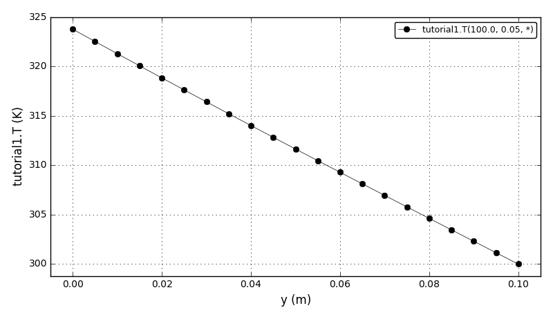
In this example we model a simple heat conduction problem: a conduction through a very thin, rectangular copper plate.
For this problem, we need a two-dimensional Cartesian grid (x,y) (here, for simplicity, divided into 10 x 10 segments):
 y axis
    ^
    |
Ly -| L T T T T T T T T T R
    | L + + + + + + + + + R
    | L + + + + + + + + + R
    | L + + + + + + + + + R
    | L + + + + + + + + + R
    | L + + + + + + + + + R
    | L + + + + + + + + + R
    | L + + + + + + + + + R
    | L + + + + + + + + + R
    | L + + + + + + + + + R
 0 -| L B B B B B B B B B R
    --|-------------------|-------> x axis
      0                   Lx
Points ‘B’ at the bottom edge of the plate (for y = 0), and the points ‘T’ at the top edge of the plate (for y = Ly) represent the points where the heat is applied.
The plate is considered insulated at the left (x = 0) and the right edges (x = Lx) of the plate (points ‘L’ and ‘R’). To model this type of problem, we have to write a heat balance equation for all interior points except the left, right, top and bottom edges, where we need to specify boundary conditions.
In this problem we have to define two distribution domains:
x (x axis, length Lx = 0.1 m)
y (y axis, length Ly = 0.1 m)
the following parameters:
rho: copper density, 8960 kg/m3
cp: copper specific heat capacity, 385 J/(kgK)
k: copper heat conductivity, 401 W/(mK)
Qb: heat flux at the bottom edge, 1E6 W/m2 (or 100 W/cm2)
Tt: temperature at the top edge, 300 K
and a single variable:
T: the temperature of the plate (distributed on x and y domains)
The model consists of 5 equations (1 distributed equation + 4 boundary conditions):
Heat balance:
rho * cp * dT(x,y)/dt = k * [d2T(x,y)/dx2 + d2T(x,y)/dy2]; x in (0, Lx), y in (0, Ly)
Neumann boundary conditions at the bottom edge:
-k * dT(x,y)/dy = Qb; x in (0, Lx), y = 0
Dirichlet boundary conditions at the top edge:
T(x,y) = Tt; x in (0, Lx), y = Ly
Neumann boundary conditions at the left edge (insulated):
dT(x,y)/dx = 0; y in [0, Ly], x = 0
Neumann boundary conditions at the right edge (insulated):
dT(x,y)/dx = 0; y in [0, Ly], x = Lx
The temperature plot (at t=100s, x=0.5, y=*):
Files
Model report |
|
Runtime model report |
|
Source code |
|
C++ source code |
1.3. Tutorial 2
This tutorial introduces the following concepts:
Arrays (discrete distribution domains)
Distributed parameters
Making equations more readable
Degrees of freedom
Setting an initial guess for variables (used by a DAE solver during an initial phase)
Print DAE solver statistics
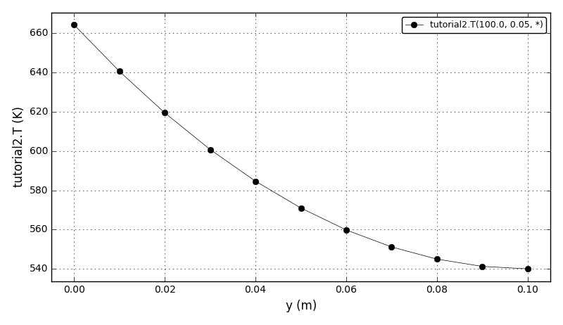
The model in this example is very similar to the model used in the tutorial 1. The differences are:
The heat capacity is temperature dependent
Different boundary conditions are applied
The temperature plot (at t=100s, x=0.5, y=*):
Files
Model report |
|
Runtime model report |
|
Source code |
|
C++ source code |
1.4. Tutorial 3
This tutorial introduces the following concepts:
Arrays of variable values
Functions that operate on arrays of values
Functions that create constants and arrays of constant values (Constant and Array)
Non-uniform domain grids
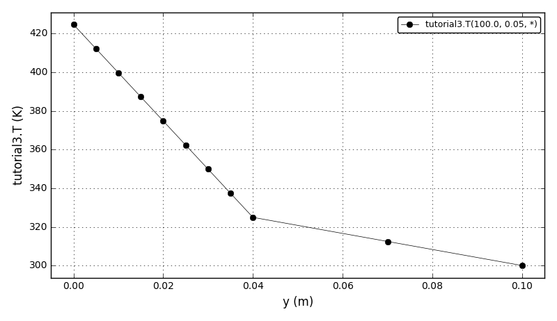
The model in this example is identical to the model used in the tutorial 1. Some additional equations that calculate the total flux at the bottom edge are added to illustrate the array functions.
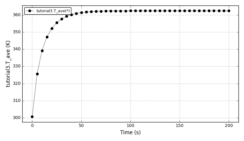
The temperature plot (at t=100, x=0.5, y=*):
The average temperature plot (considering the whole x-y domain):
Files
Model report |
|
Runtime model report |
|
Source code |
1.5. Tutorial 4
This tutorial introduces the following concepts:
Discontinuous equations (symmetrical state transition networks: daeIF statements)
Building of Jacobian expressions
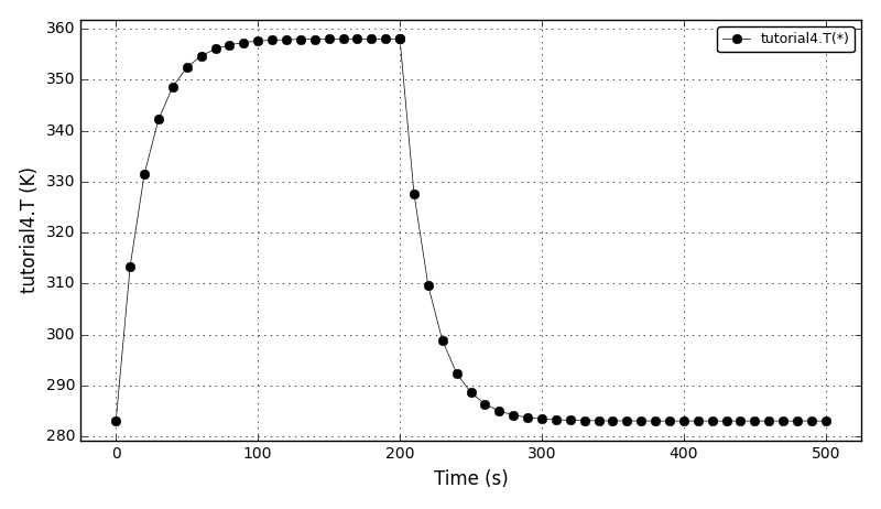
In this example we model a very simple heat transfer problem where a small piece of copper is at one side exposed to the source of heat and at the other to the surroundings.
The lumped heat balance is given by the following equation:
rho * cp * dT/dt - Qin = h * A * (T - Tsurr)
where Qin is the power of the heater, h is the heat transfer coefficient, A is the surface area and Tsurr is the temperature of the surrounding air.
The process starts at the temperature of the metal of 283K. The metal is allowed to warm up for 200 seconds, when the heat source is removed and the metal cools down slowly to the ambient temperature.
This can be modelled using the following symmetrical state transition network:
IF t < 200
  Qin = 1500 W
ELSE
  Qin = 0 W
The temperature plot:
Files
Model report |
|
Runtime model report |
|
Source code |
|
C++ source code |
1.6. Tutorial 5
This tutorial introduces the following concepts:
Discontinuous equations (non-symmetrical state transition networks: daeSTN statements)
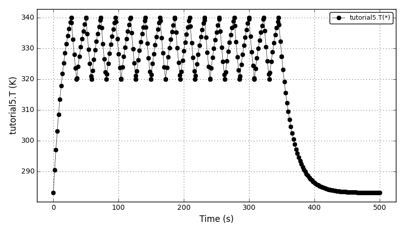
In this example we use the same heat transfer problem as in the tutorial 4. Again we have a piece of copper which is at one side exposed to the source of heat and at the other to the surroundings.
The process starts at the temperature of 283K. The metal is allowed to warm up, and then its temperature is kept in the interval (320K - 340K) for 350 seconds. This is performed by switching the heater on when the temperature drops to 320K and by switching the heater off when the temperature reaches 340K. After 350s the heat source is permanently switched off and the metal is allowed to slowly cool down to the ambient temperature.
This can be modelled using the following non-symmetrical state transition network:
STN Regulator
  case Heating:
    Qin = 1500 W
    on condition T > 340K switch to Regulator.Cooling
    on condition t > 350s switch to Regulator.HeaterOff

  case Cooling:
    Qin = 0 W
    on condition T < 320K switch to Regulator.Heating
    on condition t > 350s switch to Regulator.HeaterOff

  case HeaterOff:
    Qin = 0 W
The temperature plot:
Files
Model report |
|
Runtime model report |
|
Source code |
|
C++ source code |
1.7. Tutorial 6
This tutorial introduces the following concepts:
Ports
Port connections
Units (instances of other models)
A simple port type ‘portSimple’ is defined which contains only one variable ‘t’. Two models ‘modPortIn’ and ‘modPortOut’ are defined, each having one port of type ‘portSimple’. The wrapper model ‘modTutorial’ instantiate these two models as its units and connects them by connecting their ports.
Files
Model report |
|
Runtime model report |
|
Source code |
|
C++ source code |
1.8. Tutorial 7
This tutorial introduces the following concepts:
Quasi steady state initial condition mode (eQuasiSteadyState flag)
User-defined schedules (operating procedures)
Resetting of degrees of freedom
Resetting of initial conditions
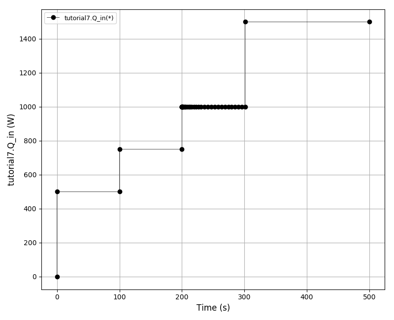
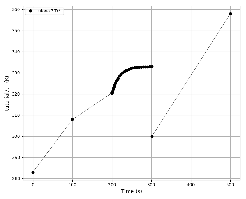
In this example we use the same heat transfer problem as in the tutorial 4. The input power of the heater is defined as a variable. Since there is no equation defined to calculate the value of the input power, the system contains N variables but only N-1 equations. To create a well-posed DAE system one of the variable needs to be “fixed”. However the choice of variables is not arbitrary and in this example the only variable that can be fixed is Qin. Thus, the Qin variable represents a degree of freedom (DOF). Its value will be fixed at the beginning of the simulation and later manipulated in the user-defined schedule in the overloaded function daeSimulation.Run().
The default daeSimulation.Run() function (re-implemented in Python) is:
def Run(self):
    # Python implementation of daeSimulation::Run() C++ function.

    import math
    while self.CurrentTime < self.TimeHorizon:
        # Get the time step (based on the TimeHorizon and the ReportingInterval).
        # Do not allow to get past the TimeHorizon.
        t = self.NextReportingTime
        if t > self.TimeHorizon:
            t = self.TimeHorizon

        # If the flag is set - a user tries to pause the simulation, therefore return.
        if self.ActivityAction == ePauseActivity:
            self.Log.Message("Activity paused by the user", 0)
            return

        # If a discontinuity is found, loop until the end of the integration period.
        # The data will be reported around discontinuities!
        while t > self.CurrentTime:
            self.Log.Message("Integrating from [%f] to [%f] ..." % (self.CurrentTime, t), 0)
            self.IntegrateUntilTime(t, eStopAtModelDiscontinuity, True)

        # After the integration period, report the data.
        self.ReportData(self.CurrentTime)

        # Set the simulation progress.
        newProgress = math.ceil(100.0 * self.CurrentTime / self.TimeHorizon)
        if newProgress > self.Log.Progress:
            self.Log.Progress = newProgress
In this example the following schedule is specified:
Re-assign the value of Qin to 500W, run the simulation for 100s using the IntegrateForTimeInterval function and report the data using the ReportData() function.
Re-assign the value of Qin to 750W, run the simulation the time reaches 200s using the IntegrateUntilTime function and report the data.
Re-assign the variable Qin to 1000W, run the simulation for 100s in OneStep mode using the IntegrateForOneStep() function and report the data at every time step.
Re-assign the variable Qin to 1500W, re-initialise the temperature again to 300K, run the simulation until the TimeHorizon is reached using the function Integrate() and report the data.
The plot of the inlet power:
The temperature plot:
Files
Model report |
|
Runtime model report |
|
Source code |
1.9. Tutorial 8
This tutorial introduces the following concepts:
Data reporters and exporting results into the following file formats:
Matlab MAT file (requires python-scipy package)
MS Excel .xls file (requires python-xlwt package)
JSON file (no third party dependencies)
VTK file (requires pyevtk and vtk packages)
XML file (requires python-lxml package)
HDF5 file (requires python-h5py package)
Pandas dataset (requires python-pandas package)
Implementation of user-defined data reporters
daeDelegateDataReporter
Some time it is not enough to send the results to the DAE Plotter but it is desirable to export them into a specified file format (i.e. for use in other programs). For that purpose, daetools provide a range of data reporters that save the simulation results in various formats. In adddition, daetools allow implementation of custom, user-defined data reporters. As an example, a user-defined data reporter is developed to save the results into a plain text file (after the simulation is finished). Obviously, the data can be processed in any other fashion. Moreover, in certain situation it is required to process the results in more than one way. The daeDelegateDataReporter can be used in those cases. It has the same interface and the functionality like all data reporters. However, it does not do any data processing itself but calls the corresponding functions of data reporters which are added to it using the function AddDataReporter. This way it is possible, at the same time, to send the results to the DAE Plotter and save them into a file (or process the data in some other ways). In this example the results are processed in 10 different ways at the same time.
The model used in this example is very similar to the model in the tutorials 4 and 5.
Files
Model report |
|
Runtime model report |
|
Source code |
1.10. Tutorial 9
This tutorial introduces the following concepts:
Third party direct linear equations solvers
Currently there are the following linear equations solvers available:
SuperLU: sequential sparse direct solver defined in pySuperLU module (BSD licence)
SuperLU_MT: multi-threaded sparse direct solver defined in pySuperLU_MT module (BSD licence)
Trilinos Amesos: sequential sparse direct solver defined in pyTrilinos module (GNU Lesser GPL)
IntelPardiso: multi-threaded sparse direct solver defined in pyIntelPardiso module (proprietary)
Pardiso: multi-threaded sparse direct solver defined in pyPardiso module (proprietary)
In this example we use the same conduction problem as in the tutorial 1.
The temperature plot (at t=100s, x=0.5, y=*):

Files
Model report |
|
Runtime model report |
|
Source code |
1.11. Tutorial 10
This tutorial introduces the following concepts:
Initialization files
Domains which bounds depend on parameter values
Evaluation of integrals
In this example we use the same conduction problem as in the tutorial 1.
Files
Model report |
|
Runtime model report |
|
Source code |
1.12. Tutorial 11
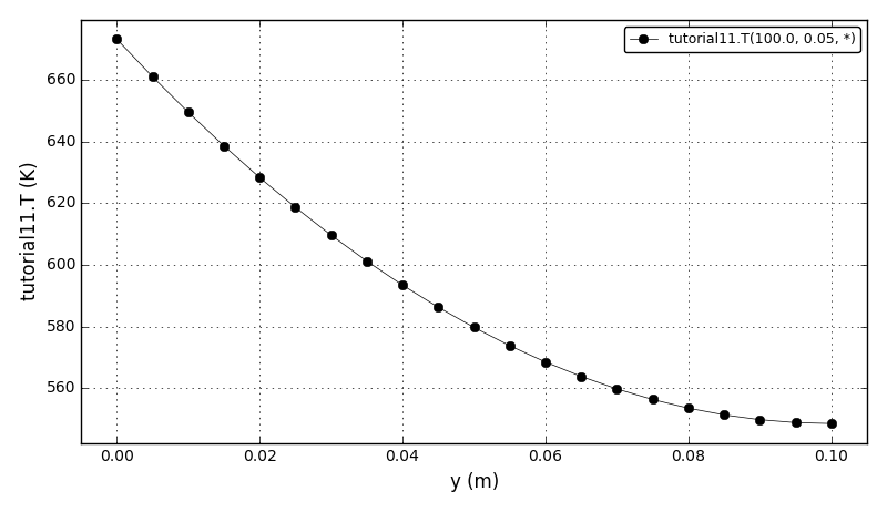
This tutorial describes the use of iterative linear solvers (AztecOO from the Trilinos project) with different preconditioners (built-in AztecOO, Ifpack or ML) and corresponding solver options. Also, the range of Trilinos Amesos solver options are shown.
The model is very similar to the model in tutorial 1, except for the different boundary conditions and that the equations are written in a different way to maximise the number of items around the diagonal (creating the problem with the diagonally dominant matrix). These type of systems can be solved using very simple preconditioners such as Jacobi. To do so, the interoperability with the NumPy package has been exploited and the package itertools used to iterate through the distribution domains in x and y directions.
The equations are distributed in such a way that the following incidence matrix is obtained:
|XXX                                 |
| X     X     X                      |
|  X     X     X                     |
|   X     X     X                    |
|    X     X     X                   |
|   XXX                              |
|      XXX                           |
| X    XXX    X                      |
|  X    XXX    X                     |
|   X    XXX    X                    |
|    X    XXX    X                   |
|         XXX                        |
|            XXX                     |
|       X    XXX    X                |
|        X    XXX    X               |
|         X    XXX    X              |
|          X    XXX    X             |
|               XXX                  |
|                  XXX               |
|             X    XXX    X          |
|              X    XXX    X         |
|               X    XXX    X        |
|                X    XXX    X       |
|                     XXX            |
|                        XXX         |
|                   X    XXX    X    |
|                    X    XXX    X   |
|                     X    XXX    X  |
|                      X    XXX    X |
|                           XXX      |
|                              XXX   |
|                   X     X     X    |
|                    X     X     X   |
|                     X     X     X  |
|                      X     X     X |
|                                 XXX|
The temperature plot (at t=100s, x=0.5, y=*):
Files
Model report |
|
Runtime model report |
|
Source code |
1.13. Tutorial 12
This tutorial describes the use and available options for superLU direct linear solvers:
Sequential: superLU
Multithreaded (OpenMP/posix threads): superLU_MT
The model is the same as the model in tutorial 1, except for the different boundary conditions.
The temperature plot (at t=100s, x=0.5, y=*):

Files
Model report |
|
Runtime model report |
|
Source code |
1.14. Tutorial 13
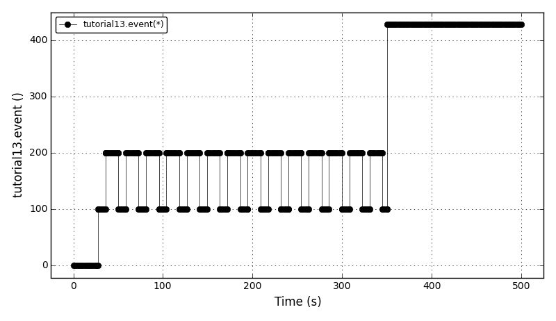
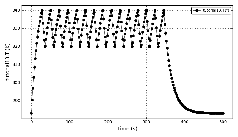
This tutorial introduces the following concepts:
The event ports
ON_CONDITION() function illustrating the types of actions that can be executed during state transitions
ON_EVENT() function illustrating the types of actions that can be executed when an event is triggered
User defined actions
In this example we use the very similar model as in the tutorial 5.
The simulation output should show the following messages at t=100s and t=350s:
...
********************************************************
simpleUserAction2 message:
This message should be fired when the time is 100s.
********************************************************
...
********************************************************
simpleUserAction executed; input data = 427.464093129832
********************************************************
...
The plot of the ‘event’ variable:
The temperature plot:
Files
Model report |
|
Runtime model report |
|
Source code |
1.15. Tutorial 14
In this tutorial we introduce the external functions concept that can handle and execute functions in external libraries. The daeScalarExternalFunction-derived external function object is used to calculate the heat transferred and to interpolate a set of values using the scipy.interpolate.interp1d object. In addition, functions defined in shared libraries (.so in GNU/Linux, .dll in Windows and .dylib in macOS) can be used via ctypes Python library and daeCTypesExternalFunction class.
In this example we use the same model as in the tutorial 5 with few additional equations.
The simulation output should show the following messages at the end of simulation:
...
scipy.interp1d statistics:
  interp1d called 1703 times (cache value used 770 times)
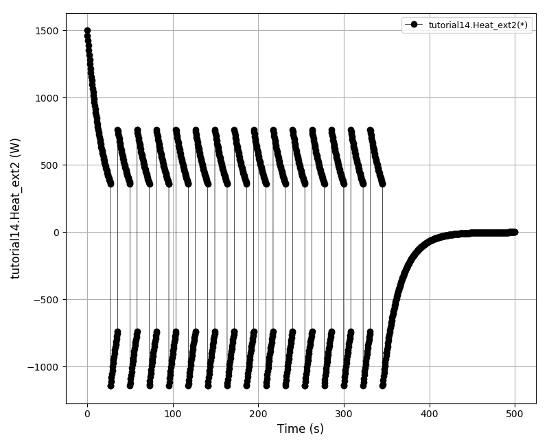
The plot of the ‘Heat_ext1’ variable:

The plot of the ‘Heat_ext2’ variable:
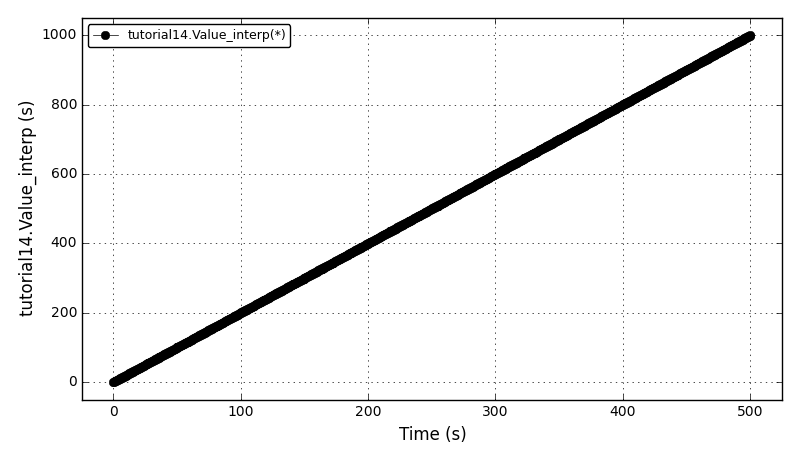
The plot of the ‘Value_interp’ variable:
Files
Model report |
|
Runtime model report |
|
Source code |
|
External function source code |
|
C++ source code |
1.16. Tutorial 15
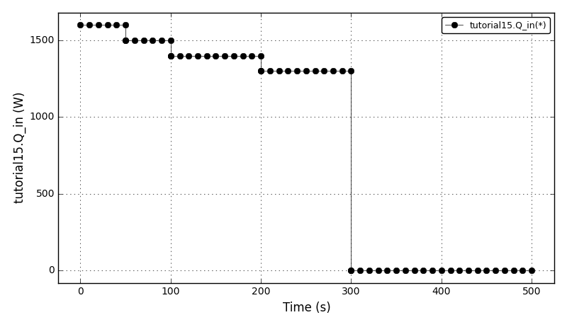
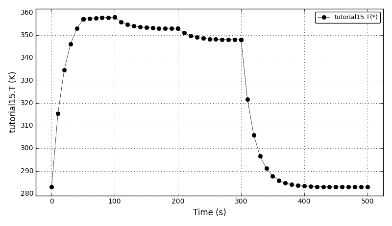
This tutorial introduces the following concepts:
Nested state transitions
In this example we use the same model as in the tutorial 4 with the more complex STN:
IF t < 200
  IF 0 <= t < 100
     IF 0 <= t < 50
       Qin = 1600 W
     ELSE
       Qin = 1500 W
  ELSE
    Qin = 1400 W

ELSE IF 200 <= t < 300
  Qin = 1300 W

ELSE
  Qin = 0 W
The plot of the ‘Qin’ variable:
The temperature plot:
Files
Model report |
|
Runtime model report |
|
Source code |
1.17. Tutorial 16
This tutorial shows how to use DAE Tools objects with NumPy arrays to solve a simple stationary heat conduction in one dimension using the Finite Elements method with linear elements and two ways of manually assembling a stiffness matrix/load vector:
d2T(x)/dx2 = F(x); x in (0, Lx)
Linear finite elements discretisation and simple FE matrix assembly:
                  phi                 phi
                     (k-1)               (k)

                    *                   *
                  * | *               * | *
                *   |   *           *   |   *
              *     |     *       *     |     *
            *       |       *   *       |       *
          *         |         *         |         *
        *           |       *   *       |           *
      *             |     *       *     |             *
    *               |   *           *   |               *
  *                 | *  element (k)  * |                 *
*-------------------*+++++++++++++++++++*-------------------*-
                    x                   x
                     (k-i                (k)

                    \_________ _________/
                              |
                              dx
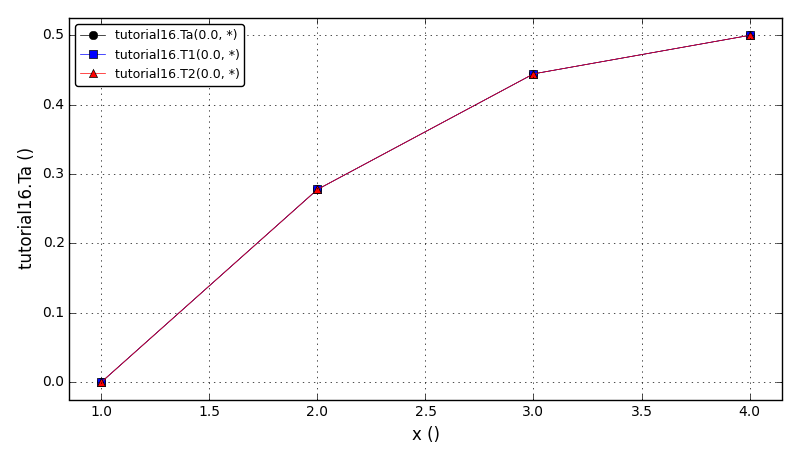
The comparison of the analytical solution and two ways of assembling the system is given in the following plot:
Files
Model report |
|
Runtime model report |
|
Source code |
1.18. Tutorial 17
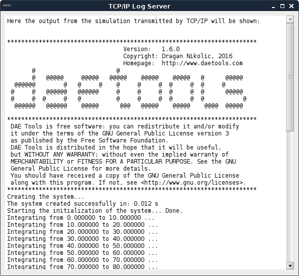
This tutorial introduces the following concepts:
TCPIP Log and TCPIPLogServer
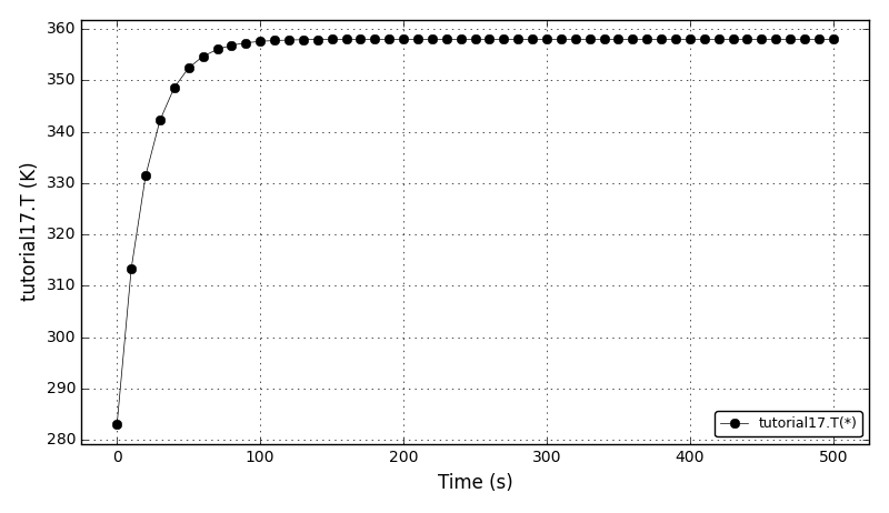
In this example we use the same heat transfer problem as in the tutorial 7.
The screenshot of the TCP/IP log server:
The temperature plot:
Files
Model report |
|
Runtime model report |
|
Source code |
1.19. Tutorial 18
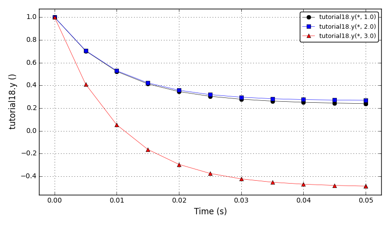
This tutorial shows one more problem solved using the NumPy arrays that operate on DAE Tools variables. The model is taken from the Sundials ARKODE (ark_analytic_sys.cpp). The ODE system is defined by the following system of equations:
dy/dt = A*y
where:
A = V * D * Vi
V = [1 -1 1; -1 2 1; 0 -1 2];
Vi = 0.25 * [5 1 -3; 2 2 -2; 1 1 1];
D = [-0.5 0 0; 0 -0.1 0; 0 0 lam];
lam is a large negative number.
The analytical solution to this problem is:
Y(t) = V*exp(D*t)*Vi*Y0
for t in the interval [0.0, 0.05], with initial condition y(0) = [1,1,1]’.
The stiffness of the problem is directly proportional to the value of “lamda”. The value of lamda should be negative to result in a well-posed ODE; for values with magnitude larger than 100 the problem becomes quite stiff.
In this example, we choose lamda = -100.
The solution:
lamda = -100
reltol = 1e-06
abstol = 1e-10

--------------------------------------
   t        y0        y1        y2
--------------------------------------
 0.0050   0.70327   0.70627   0.41004
 0.0100   0.52267   0.52865   0.05231
 0.0150   0.41249   0.42145  -0.16456
 0.0200   0.34504   0.35696  -0.29600
 0.0250   0.30349   0.31838  -0.37563
 0.0300   0.27767   0.29551  -0.42383
 0.0350   0.26138   0.28216  -0.45296
 0.0400   0.25088   0.27459  -0.47053
 0.0450   0.24389   0.27053  -0.48109
 0.0500   0.23903   0.26858  -0.48740
--------------------------------------
The plot of the ‘y0’, ‘y1’, ‘y2’ variables:
Files
Model report |
|
Runtime model report |
|
Source code |
1.20. Tutorial 19
This tutorial introduces the thermo physical property packages.
Since there are many thermo packages with a very different API the CapeOpen standard has been adopted in daetools. This way, all thermo packages implementing the CapeOpen thermo interfaces are automatically vailable to daetools. Those which do not are wrapped by the class with the CapeOpen conforming API. At the moment, two types of thermophysical property packages are implemented:
Any CapeOpen v1.1 thermo package (available only in Windows)
CoolProp thermo package (available for all platforms) wrapped in the class with the CapeOpen interface.
The central point is the daeThermoPhysicalPropertyPackage class. It can load any COM component that implements CapeOpen 1.1 ICapeThermoPropertyPackageManager interface or the CoolProp thermo package.
The framework provides low-level functions (specified in the CapeOpen standard) in the daeThermoPhysicalPropertyPackage class and the higher-level functions in the auxiliary daeThermoPackage class defined in the daetools/pyDAE/thermo_packages.py file. The low-level functions are defined in the ICapeThermoCoumpounds and ICapeThermoPropertyRoutine CapeOpen interfaces. These functions come in two flavours:
The ordinary functions return adouble/adouble_array objects and can only be used to specify equations:
GetCompoundConstant (from ICapeThermoCoumpounds interface)
GetTDependentProperty (from ICapeThermoCoumpounds interface)
GetPDependentProperty (from ICapeThermoCoumpounds interface)
CalcSinglePhaseScalarProperty (from ICapeThermoPropertyRoutine interface: scalar version)
CalcSinglePhaseVectorProperty (from ICapeThermoPropertyRoutine interface: vector version)
CalcTwoPhaseScalarProperty (from ICapeThermoPropertyRoutine interface: scalar version)
CalcTwoPhaseVectorProperty (from ICapeThermoPropertyRoutine interface: vector version)
The functions starting with the underscores can be used for calculations (they use and return float values):
_GetCompoundConstant
_GetTDependentProperty
_GetPDependentProperty
_CalcSinglePhaseScalarProperty
_CalcSinglePhaseVectorProperty
_CalcTwoPhaseScalarProperty
_CalcTwoPhaseVectorProperty
The daeThermoPackage auxiliary class offers functions to calculate specified properties, for instance:
Transport properties:
cp, kappa, mu, Dab (heat capacity, thermal conductivity, dynamic viscosity, diffusion coefficient)
Thermodynamic properties:
rho
h, s, G, H, I (enthalpy, entropy, gibbs/helmholtz/internal energy)
h_E, s_E, G_E, H_E, I_E, V_E (excess enthalpy, entropy, gibbs/helmholtz/internal energy, volume)
f and phi (fugacity and coefficient of fugacity)
a and gamma (activity and the coefficient of activity)
z (compressibility factor)
K, surfaceTension (ratio of fugacity coefficients and the surface tension)
- Nota bene:
Some of the above functions return scalars while the others return arrays of values. Check the thermo_packages.py file for details.
All functions return properties in the SI units (as specified in the CapeOpen 1.1 standard).
Known issues:
Many properties from the CapeOpen standard are not supported by all thermo packages.
CalcEquilibrium from the ICapeThermoEquilibriumRoutine is not supported.
CoolProp does not provide transport models for many compounds.
The function calls are NOT thread safe.
The code generation will NOT work for models using the thermo packages.
Some CapeOpen thermo packags refuse to return properties for mass basis (i.e. density).
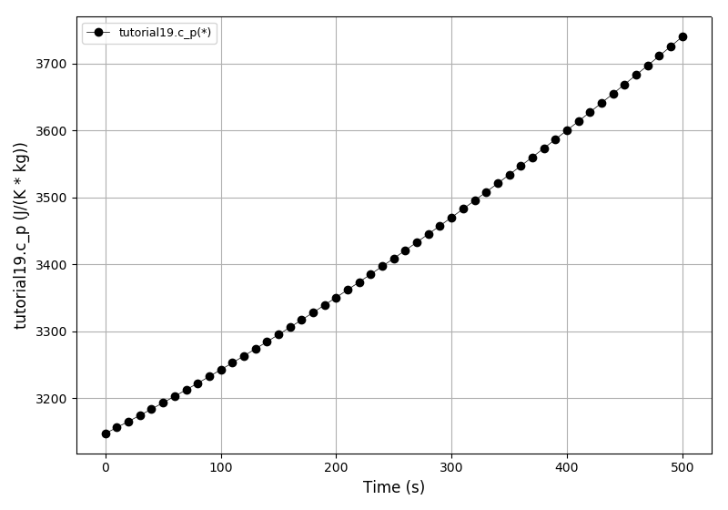
In this tutorial, we use a very simple model: a quantity of liquid (water + ethanol mixture) is heated using the constant input power. The model uses a thermo package to calculate the commonly used transport properties such as specific heat capacity, thermal conductivity, dynamic viscosity and binary diffusion coefficients. First, the low-level functions are tested for CapeOpen and CoolProp packages in the test_single_phase, test_two_phase, test_coolprop_single_phase functions. The results depend on the options selected in the CapeOpen package (equation of state, etc.). Then, the model that uses a thermo package is simulated.
The plot of the specific heat capacity as a function of temperature:
- Nota bene:
There is a difference between results in Windows and other platforms since the CapeOpen thermo packages are available only in Windows.
Files
Model report |
|
Runtime model report |
|
Source code |
1.21. Tutorial 20
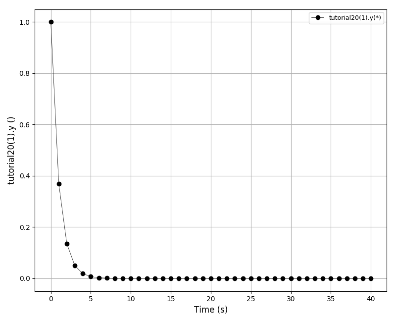
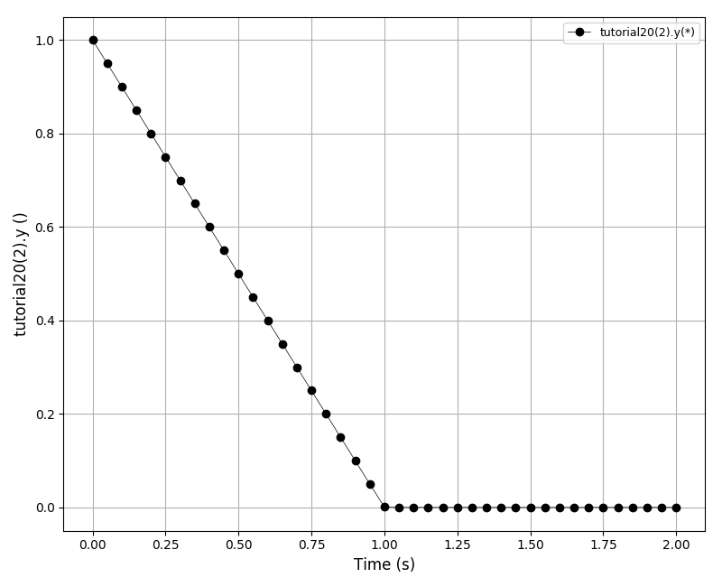
This tutorial illustrates the support variable constraints available in Sundials IDA solver. Benchmarks are available from Matlab documentation.
Absolute Value Function:
dy/dt = -fabs(y)
solved on the interval [0,40] with the initial condition y(0) = 1. The solution of this ODE decays to zero. If the solver produces a negative solution value, the computation eventually will fail as the calculated solution diverges to -inf. Using the constraint y >= 0 resolves this problem.
The Knee problem:
epsilon * dy/dt = (1-t)*y - y**2
solved on the interval [0,2] with the initial condition y(0) = 1. The parameter epsilon is 0 < epsilon << 1 and in this example equal to 1e-6. The solution follows the y = 1-x isocline for the whole interval of integration which is incorrect. Using the constraint y >= 0 resolves the problem.
In DAE Tools contraints follow the Sundials IDA solver implementation and can be specified using the valueConstraint argument of the daeVariableType class __init__ function:
eNoConstraint (default)
eValueGTEQ: imposes >= 0 constraint
eValueLTEQ: imposes <= 0 constraint
eValueGT: imposes > 0 constraint
eValueLT: imposes < 0 constraint
and changed for individual variables using daeVariable.SetValueConstraint functions.
Absolute Value Function solution plot:
The Knee problem solution plot:
Files
Source code |
1.22. Tutorial 21
This tutorial introduces different methods for evaluation of equations in parallel. Equations residuals, Jacobian matrix and sensitivity residuals can be evaluated in parallel using two methods
The Evaluation Tree approach (default)
OpenMP API is used for evaluation in parallel. This method is specified by setting daetools.core.equations.evaluationMode option in daetools.cfg to “evaluationTree_OpenMP” or setting the simulation property:
simulation.EvaluationMode = eEvaluationTree_OpenMP
numThreads controls the number of OpenMP threads in a team. If numThreads is 0 the default number of threads is used (the number of cores in the system). Sequential evaluation is achieved by setting numThreads to 1.
The Compute Stack approach
Equations can be evaluated in parallel using:
OpenMP API for general purpose processors and manycore devices.
This method is specified by setting daetools.core.equations.evaluationMode option in daetools.cfg to “computeStack_OpenMP” or setting the simulation property:
simulation.EvaluationMode = eComputeStack_OpenMP
numThreads controls the number of OpenMP threads in a team. If numThreads is 0 the default number of threads is used (the number of cores in the system). Sequential evaluation is achieved by setting numThreads to 1.
OpenCL framework for streaming processors and heterogeneous systems.
This type is implemented in an external Python module pyEvaluator_OpenCL. It is up to one order of magnitude faster than the Evaluation Tree approach. However, it does not support external functions nor thermo-physical packages.
OpenCL evaluators can use a single or multiple OpenCL devices. It is required to install OpenCL drivers/runtime libraries. Intel: https://software.intel.com/en-us/articles/opencl-drivers AMD: https://support.amd.com/en-us/kb-articles/Pages/OpenCL2-Driver.aspx NVidia: https://developer.nvidia.com/opencl
Files
Source code |