All Tutorials

What’s the time? (AKA: Hello world!)

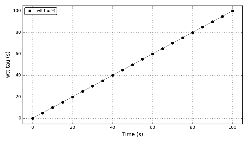
What is the time? (AKA Hello world!) is a very simple model. The model consists of a single variable (called ‘time’) and a single differential equation:

d(time)/dt = 1

This way, the value of the variable ‘time’ is equal to the elapsed time in the simulation.

This tutorial presents the basic structure of daeModel and daeSimulation classes. A typical DAETools simulation requires the following 8 tasks:

1. Importing DAE Tools pyDAE module(s)

2. Importing or declaration of units and variable types (unit and daeVariableType classes)

3. Developing a model by deriving a class from the base daeModel class and:

   • Declaring domains, parameters and variables in the daeModel.__init__ function

   • Declaring equations and their residual expressions in the daeModel.DeclareEquations function

4. Setting up a simulation by deriving a class from the base daeSimulation class and:

   • Specifying a model to be used in the simulation in the daeSimulation.__init__ function

   • Setting the values of parameters in the daeSimulation.SetUpParametersAndDomains function

   • Setting initial conditions in the daeSimulation.SetUpVariables function

5. Declaring auxiliary objects required for the simulation

   • DAE solver object

   • Data reporter object

   • Log object

6. Setting the run-time options for the simulation:

   • ReportingInterval

   • TimeHorizon

7. Connecting a data reporter

8. Initializing, running and finalizing the simulation

The ‘time’ variable plot:

Files

Model report	whats_the_time.xml
Runtime model report	whats_the_time-rt.xml
Source code	whats_the_time.py
C++ source code	whats_the_time.cpp

Tutorial 1

This tutorial introduces several new concepts:

• Distribution domains

• Distributed parameters, variables and equations

• Setting boundary conditions (Neumann and Dirichlet type)

• Setting initial conditions

In this example we model a simple heat conduction problem: a conduction through a very thin, rectangular copper plate.

For this problem, we need a two-dimensional Cartesian grid (x,y) (here, for simplicity, divided into 10 x 10 segments):

 y axis
    ^
    |
Ly -| L T T T T T T T T T R
    | L + + + + + + + + + R
    | L + + + + + + + + + R
    | L + + + + + + + + + R
    | L + + + + + + + + + R
    | L + + + + + + + + + R
    | L + + + + + + + + + R
    | L + + + + + + + + + R
    | L + + + + + + + + + R
    | L + + + + + + + + + R
 0 -| L B B B B B B B B B R
    --|-------------------|-------> x axis
      0                   Lx

Points ‘B’ at the bottom edge of the plate (for y = 0), and the points ‘T’ at the top edge of the plate (for y = Ly) represent the points where the heat is applied.

The plate is considered insulated at the left (x = 0) and the right edges (x = Lx) of the plate (points ‘L’ and ‘R’). To model this type of problem, we have to write a heat balance equation for all interior points except the left, right, top and bottom edges, where we need to specify boundary conditions.

In this problem we have to define two distribution domains:

• x (x axis, length Lx = 0.1 m)

• y (y axis, length Ly = 0.1 m)

the following parameters:

• rho: copper density, 8960 kg/m3

• cp: copper specific heat capacity, 385 J/(kgK)

• k: copper heat conductivity, 401 W/(mK)

• Qb: heat flux at the bottom edge, 1E6 W/m2 (or 100 W/cm2)

• Tt: temperature at the top edge, 300 K

and a single variable:

• T: the temperature of the plate (distributed on x and y domains)

The model consists of 5 equations (1 distributed equation + 4 boundary conditions):

1. Heat balance:

   rho * cp * dT(x,y)/dt = k * [d2T(x,y)/dx2 + d2T(x,y)/dy2];  x in (0, Lx), y in (0, Ly)
   

2. Neumann boundary conditions at the bottom edge:

   -k * dT(x,y)/dy = Qb;  x in (0, Lx), y = 0
   

3. Dirichlet boundary conditions at the top edge:

   T(x,y) = Tt;  x in (0, Lx), y = Ly
   

4. Neumann boundary conditions at the left edge (insulated):

   dT(x,y)/dx = 0;  y in [0, Ly], x = 0
   

5. Neumann boundary conditions at the right edge (insulated):

   dT(x,y)/dx = 0;  y in [0, Ly], x = Lx
   

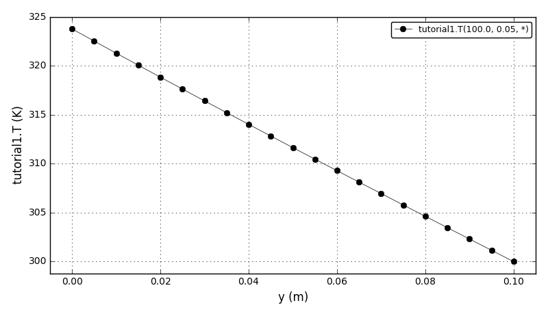
The temperature plot (at t=100s, x=0.5, y=*):

Files

Model report	tutorial1.xml
Runtime model report	tutorial1-rt.xml
Source code	tutorial1.py
C++ source code	tutorial1.cpp

Tutorial 2

This tutorial introduces the following concepts:

• Arrays (discrete distribution domains)

• Distributed parameters

• Making equations more readable

• Degrees of freedom

• Setting an initial guess for variables (used by a DAE solver during an initial phase)

• Print DAE solver statistics

The model in this example is very similar to the model used in the tutorial 1. The differences are:

• The heat capacity is temperature dependent

• Different boundary conditions are applied

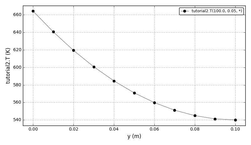
The temperature plot (at t=100s, x=0.5, y=*):

Files

Model report	tutorial2.xml
Runtime model report	tutorial2-rt.xml
Source code	tutorial2.py
C++ source code	tutorial2.cpp

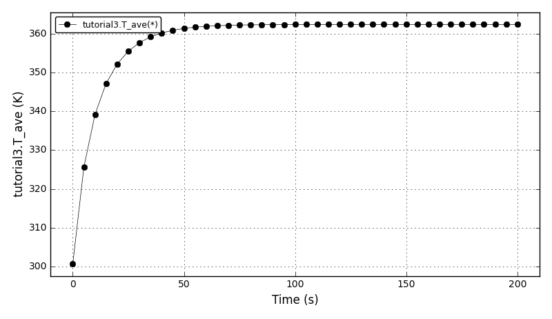
Tutorial 3

This tutorial introduces the following concepts:

• Arrays of variable values

• Functions that operate on arrays of values

• Functions that create constants and arrays of constant values (Constant and Array)

• Non-uniform domain grids

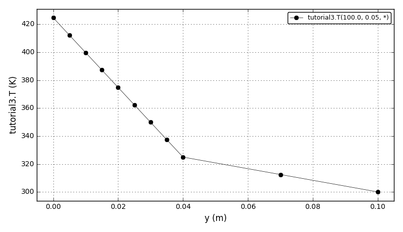
The model in this example is identical to the model used in the tutorial 1. Some additional equations that calculate the total flux at the bottom edge are added to illustrate the array functions.

The temperature plot (at t=100, x=0.5, y=*):

The average temperature plot (considering the whole x-y domain):

Files

Model report	tutorial3.xml
Runtime model report	tutorial3-rt.xml
Source code	tutorial3.py

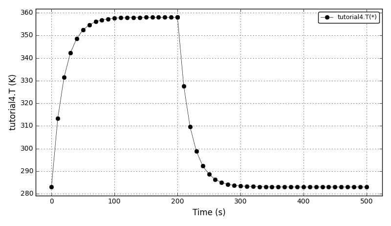
Tutorial 4

This tutorial introduces the following concepts:

• Discontinuous equations (symmetrical state transition networks: daeIF statements)

• Building of Jacobian expressions

In this example we model a very simple heat transfer problem where a small piece of copper is at one side exposed to the source of heat and at the other to the surroundings.

The lumped heat balance is given by the following equation:

rho * cp * dT/dt - Qin = h * A * (T - Tsurr)

where Qin is the power of the heater, h is the heat transfer coefficient, A is the surface area and Tsurr is the temperature of the surrounding air.

The process starts at the temperature of the metal of 283K. The metal is allowed to warm up for 200 seconds, when the heat source is removed and the metal cools down slowly to the ambient temperature.

This can be modelled using the following symmetrical state transition network:

IF t < 200
  Qin = 1500 W
ELSE
  Qin = 0 W

The temperature plot:

Files

Model report	tutorial4.xml
Runtime model report	tutorial4-rt.xml
Source code	tutorial4.py
C++ source code	tutorial4.cpp

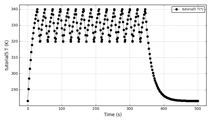
Tutorial 5

This tutorial introduces the following concepts:

• Discontinuous equations (non-symmetrical state transition networks: daeSTN statements)

In this example we use the same heat transfer problem as in the tutorial 4. Again we have a piece of copper which is at one side exposed to the source of heat and at the other to the surroundings.

The process starts at the temperature of 283K. The metal is allowed to warm up, and then its temperature is kept in the interval (320K - 340K) for 350 seconds. This is performed by switching the heater on when the temperature drops to 320K and by switching the heater off when the temperature reaches 340K. After 350s the heat source is permanently switched off and the metal is allowed to slowly cool down to the ambient temperature.

This can be modelled using the following non-symmetrical state transition network:

STN Regulator
  case Heating:
    Qin = 1500 W
    on condition T > 340K switch to Regulator.Cooling
    on condition t > 350s switch to Regulator.HeaterOff

  case Cooling:
    Qin = 0 W
    on condition T < 320K switch to Regulator.Heating
    on condition t > 350s switch to Regulator.HeaterOff

  case HeaterOff:
    Qin = 0 W

The temperature plot:

Files

Model report	tutorial5.xml
Runtime model report	tutorial5-rt.xml
Source code	tutorial5.py
C++ source code	tutorial5.cpp

Tutorial 6

This tutorial introduces the following concepts:

• Ports

• Port connections

• Units (instances of other models)

A simple port type ‘portSimple’ is defined which contains only one variable ‘t’. Two models ‘modPortIn’ and ‘modPortOut’ are defined, each having one port of type ‘portSimple’. The wrapper model ‘modTutorial’ instantiate these two models as its units and connects them by connecting their ports.

Files

Model report	tutorial6.xml
Runtime model report	tutorial6-rt.xml
Source code	tutorial6.py
C++ source code	tutorial6.cpp

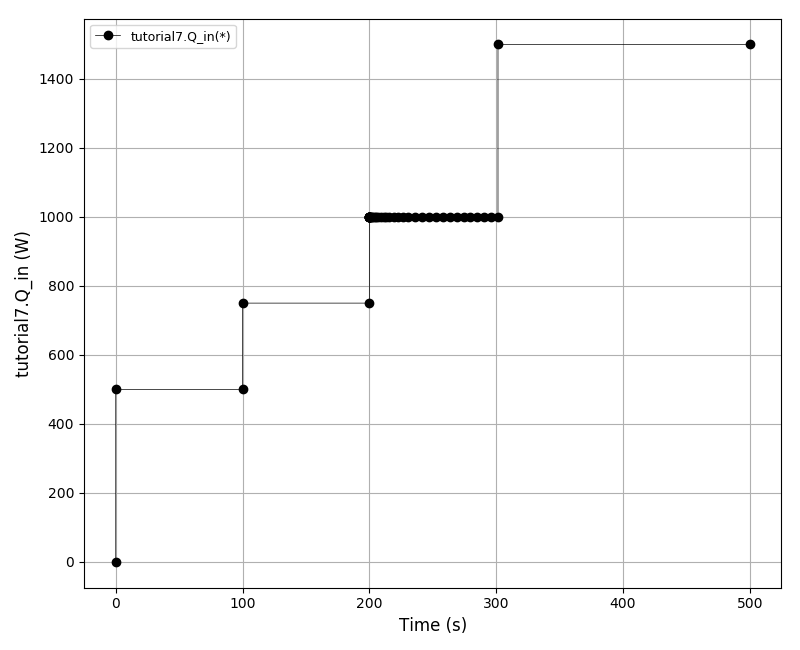
Tutorial 7

This tutorial introduces the following concepts:

• Quasi steady state initial condition mode (eQuasiSteadyState flag)

• User-defined schedules (operating procedures)

• Resetting of degrees of freedom

• Resetting of initial conditions

In this example we use the same heat transfer problem as in the tutorial 4. The input power of the heater is defined as a variable. Since there is no equation defined to calculate the value of the input power, the system contains N variables but only N-1 equations. To create a well-posed DAE system one of the variable needs to be “fixed”. However the choice of variables is not arbitrary and in this example the only variable that can be fixed is Qin. Thus, the Qin variable represents a degree of freedom (DOF). Its value will be fixed at the beginning of the simulation and later manipulated in the user-defined schedule in the overloaded function daeSimulation.Run().

The default daeSimulation.Run() function (re-implemented in Python) is:

def Run(self):
    # Python implementation of daeSimulation::Run() C++ function.

    import math
    while self.CurrentTime < self.TimeHorizon:
        # Get the time step (based on the TimeHorizon and the ReportingInterval).
        # Do not allow to get past the TimeHorizon.
        t = self.NextReportingTime
        if t > self.TimeHorizon:
            t = self.TimeHorizon

        # If the flag is set - a user tries to pause the simulation, therefore return.
        if self.ActivityAction == ePauseActivity:
            self.Log.Message("Activity paused by the user", 0)
            return

        # If a discontinuity is found, loop until the end of the integration period.
        # The data will be reported around discontinuities!
        while t > self.CurrentTime:
            self.Log.Message("Integrating from [%f] to [%f] ..." % (self.CurrentTime, t), 0)
            self.IntegrateUntilTime(t, eStopAtModelDiscontinuity, True)

        # After the integration period, report the data. 
        self.ReportData(self.CurrentTime)

        # Set the simulation progress.
        newProgress = math.ceil(100.0 * self.CurrentTime / self.TimeHorizon)
        if newProgress > self.Log.Progress:
            self.Log.Progress = newProgress

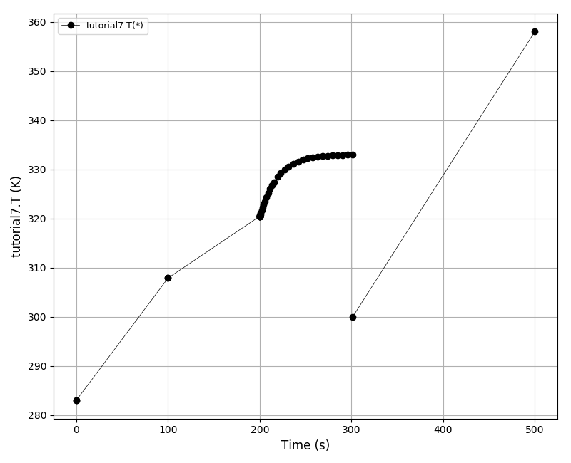
In this example the following schedule is specified:

1. Re-assign the value of Qin to 500W, run the simulation for 100s using the IntegrateForTimeInterval function and report the data using the ReportData() function.

2. Re-assign the value of Qin to 7500W, run the simulation the time reaches 200s using the IntegrateUntilTime function and report the data.

3. Re-assign the variable Qin to 1000W, run the simulation for 100s in OneStep mode using the IntegrateForOneStep() function and report the data at every time step.

4. Re-assign the variable Qin to 1500W, re-initialise the temperature again to 300K, run the simulation until the TimeHorizon is reached using the function Integrate() and report the data.

The plot of the inlet power:

The temperature plot:

Files

Model report	tutorial7.xml
Runtime model report	tutorial7-rt.xml
Source code	tutorial7.py

Tutorial 8

This tutorial introduces the following concepts:

• Data reporters and exporting results into the following file formats:

  • Matlab MAT file (requires python-scipy package)

  • MS Excel .xls file (requires python-xlwt package)

  • JSON file (no third party dependencies)

  • VTK file (requires pyevtk and vtk packages)

  • XML file (requires python-lxml package)

  • HDF5 file (requires python-h5py package)

  • Pandas dataset (requires python-pandas package)

• Implementation of user-defined data reporters

• daeDelegateDataReporter

Some time it is not enough to send the results to the DAE Plotter but it is desirable to export them into a specified file format (i.e. for use in other programs). For that purpose, daetools provide a range of data reporters that save the simulation results in various formats. In adddition, daetools allow implementation of custom, user-defined data reporters. As an example, a user-defined data reporter is developed to save the results into a plain text file (after the simulation is finished). Obviously, the data can be processed in any other fashion. Moreover, in certain situation it is required to process the results in more than one way. The daeDelegateDataReporter can be used in those cases. It has the same interface and the functionality like all data reporters. However, it does not do any data processing itself but calls the corresponding functions of data reporters which are added to it using the function AddDataReporter. This way it is possible, at the same time, to send the results to the DAE Plotter and save them into a file (or process the data in some other ways). In this example the results are processed in 10 different ways at the same time.

The model used in this example is very similar to the model in the tutorials 4 and 5.

Files

Model report	tutorial8.xml
Runtime model report	tutorial8-rt.xml
Source code	tutorial8.py

Tutorial 9

This tutorial introduces the following concepts:

• Third party direct linear equations solvers

Currently there are the following linear equations solvers available:

• SuperLU: sequential sparse direct solver defined in pySuperLU module (BSD licence)

• SuperLU_MT: multi-threaded sparse direct solver defined in pySuperLU_MT module (BSD licence)

• Trilinos Amesos: sequential sparse direct solver defined in pyTrilinos module (GNU Lesser GPL)

• IntelPardiso: multi-threaded sparse direct solver defined in pyIntelPardiso module (proprietary)

• Pardiso: multi-threaded sparse direct solver defined in pyPardiso module (proprietary)

In this example we use the same conduction problem as in the tutorial 1.

The temperature plot (at t=100s, x=0.5, y=*):

Files

Model report	tutorial9.xml
Runtime model report	tutorial9-rt.xml
Source code	tutorial9.py

Tutorial 10

This tutorial introduces the following concepts:

• Initialization files

• Domains which bounds depend on parameter values

• Evaluation of integrals

In this example we use the same conduction problem as in the tutorial 1.

Files

Model report	tutorial10.xml
Runtime model report	tutorial10-rt.xml
Source code	tutorial10.py

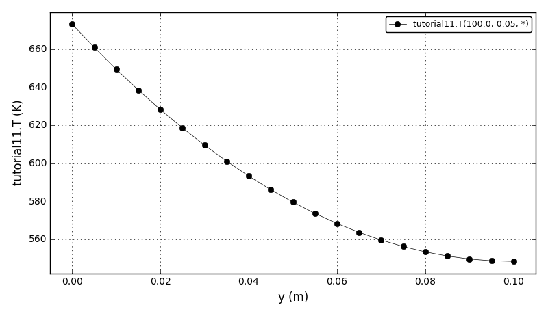
Tutorial 11

This tutorial describes the use of iterative linear solvers (AztecOO from the Trilinos project) with different preconditioners (built-in AztecOO, Ifpack or ML) and corresponding solver options. Also, the range of Trilins Amesos solver options are shown.

The model is very similar to the model in tutorial 1, except for the different boundary conditions and that the equations are written in a different way to maximise the number of items around the diagonal (creating the problem with the diagonally dominant matrix). These type of systems can be solved using very simple preconditioners such as Jacobi. To do so, the interoperability with the NumPy package has been exploited and the package itertools used to iterate through the distribution domains in x and y directions.

The equations are distributed in such a way that the following incidence matrix is obtained:

|XXX                                 |
| X     X     X                      |
|  X     X     X                     |
|   X     X     X                    |
|    X     X     X                   |
|   XXX                              |
|      XXX                           |
| X    XXX    X                      |
|  X    XXX    X                     |
|   X    XXX    X                    |
|    X    XXX    X                   |
|         XXX                        |
|            XXX                     |
|       X    XXX    X                |
|        X    XXX    X               |
|         X    XXX    X              |
|          X    XXX    X             |
|               XXX                  |
|                  XXX               |
|             X    XXX    X          |
|              X    XXX    X         |
|               X    XXX    X        |
|                X    XXX    X       |
|                     XXX            |
|                        XXX         |
|                   X    XXX    X    |
|                    X    XXX    X   |
|                     X    XXX    X  |
|                      X    XXX    X |
|                           XXX      |
|                              XXX   |
|                   X     X     X    |
|                    X     X     X   |
|                     X     X     X  |
|                      X     X     X |
|                                 XXX|

The temperature plot (at t=100s, x=0.5, y=*):

Files

Model report	tutorial11.xml
Runtime model report	tutorial11-rt.xml
Source code	tutorial11.py

Tutorial 12

This tutorial describes the use and available options for superLU direct linear solvers:

• Sequential: superLU

• Multithreaded (OpenMP/posix threads): superLU_MT

The model is the same as the model in tutorial 1, except for the different boundary conditions.

The temperature plot (at t=100s, x=0.5, y=*):

Files

Model report	tutorial12.xml
Runtime model report	tutorial12-rt.xml
Source code	tutorial12.py

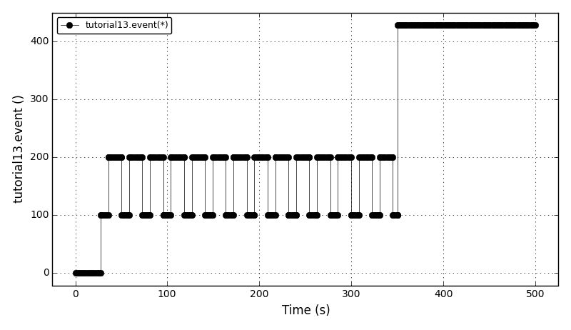
Tutorial 13

This tutorial introduces the following concepts:

• The event ports

• ON_CONDITION() function illustrating the types of actions that can be executed during state transitions

• ON_EVENT() function illustrating the types of actions that can be executed when an event is triggered

• User defined actions

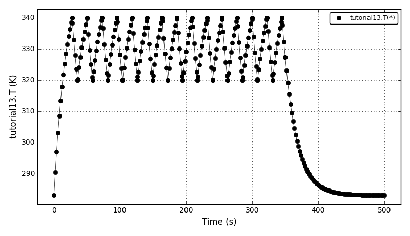
In this example we use the very similar model as in the tutorial 5.

The simulation output should show the following messages at t=100s and t=350s:

...
********************************************************
simpleUserAction2 message:
This message should be fired when the time is 100s.
********************************************************
...
********************************************************
simpleUserAction executed; input data = 427.464093129832
********************************************************
...

The plot of the ‘event’ variable:

The temperature plot:

Files

Model report	tutorial13.xml
Runtime model report	tutorial13-rt.xml
Source code	tutorial13.py

Tutorial 14

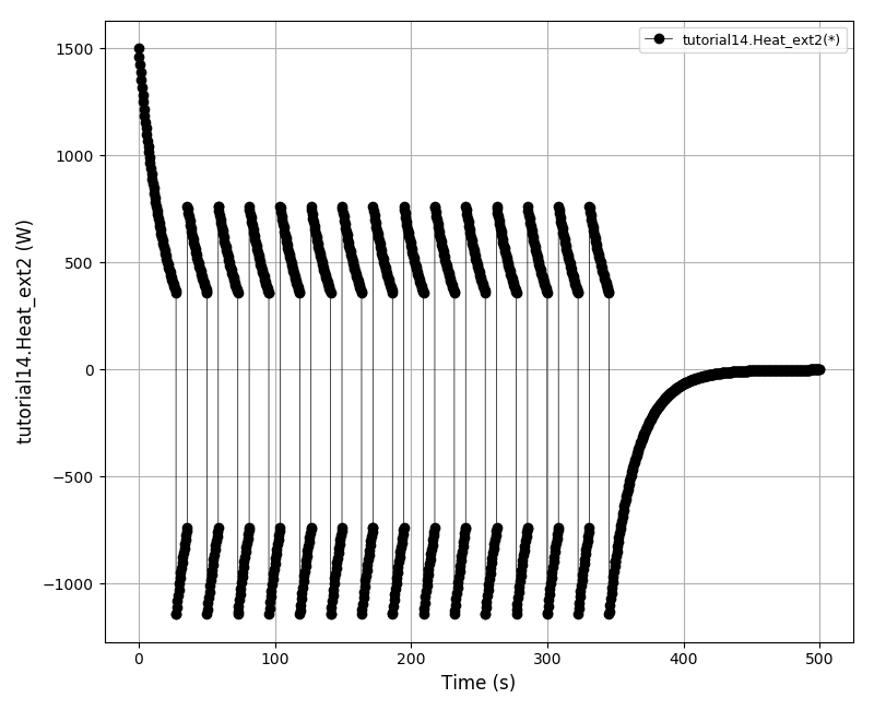
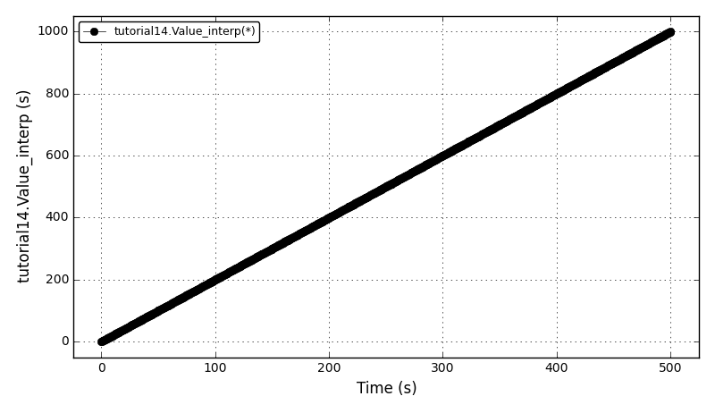
In this tutorial we introduce the external functions concept that can handle and execute functions in external libraries. The daeScalarExternalFunction-derived external function object is used to calculate the heat transferred and to interpolate a set of values using the scipy.interpolate.interp1d object. In addition, functions defined in shared libraries (.so in GNU/Linux, .dll in Windows and .dylib in macOS) can be used via ctypes Python library and daeCTypesExternalFunction class.

In this example we use the same model as in the tutorial 5 with few additional equations.

The simulation output should show the following messages at the end of simulation:

...
scipy.interp1d statistics:
  interp1d called 1703 times (cache value used 770 times)

The plot of the ‘Heat_ext1’ variable:

The plot of the ‘Heat_ext2’ variable:

The plot of the ‘Value_interp’ variable:

Files

Model report	tutorial14.xml
Runtime model report	tutorial14-rt.xml
Source code	tutorial14.py
External function source code	tutorial14_heat_function.c
C++ source code	tutorial14.cpp

Tutorial 15

This tutorial introduces the following concepts:

• Nested state transitions

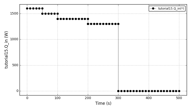
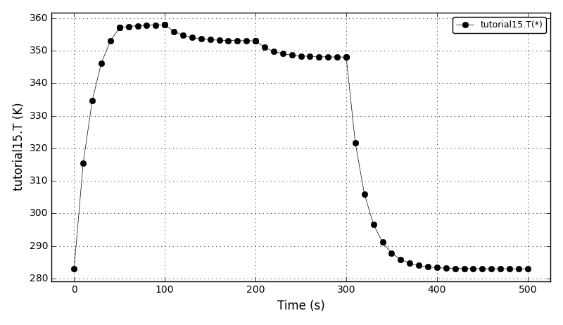
In this example we use the same model as in the tutorial 4 with the more complex STN:

IF t < 200
  IF 0 <= t < 100
     IF 0 <= t < 50
       Qin = 1600 W
     ELSE
       Qin = 1500 W
  ELSE
    Qin = 1400 W

ELSE IF 200 <= t < 300
  Qin = 1300 W

ELSE
  Qin = 0 W

The plot of the ‘Qin’ variable:

The temperature plot:

Files

Model report	tutorial15.xml
Runtime model report	tutorial15-rt.xml
Source code	tutorial15.py

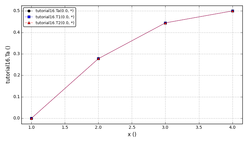
Tutorial 16

This tutorial shows how to use DAE Tools objects with NumPy arrays to solve a simple stationary heat conduction in one dimension using the Finite Elements method with linear elements and two ways of manually assembling a stiffness matrix/load vector:

d2T(x)/dx2 = F(x);  x in (0, Lx)

Linear finite elements discretisation and simple FE matrix assembly:

                  phi                 phi
                     (k-1)               (k)

                    *                   *             
                  * | *               * | *            
                *   |   *           *   |   *          
              *     |     *       *     |     *        
            *       |       *   *       |       *      
          *         |         *         |         *        
        *           |       *   *       |           *      
      *             |     *       *     |             *    
    *               |   *           *   |               *  
  *                 | *  element (k)  * |                 *
*-------------------*+++++++++++++++++++*-------------------*-
                    x                   x
                     (k-i                (k)

                    \_________ _________/
                              |
                              dx

The comparison of the analytical solution and two ways of assembling the system is given in the following plot:

Files

Model report	tutorial16.xml
Runtime model report	tutorial16-rt.xml
Source code	tutorial16.py

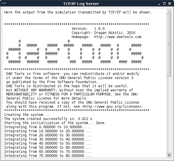
Tutorial 17

This tutorial introduces the following concepts:

• TCPIP Log and TCPIPLogServer

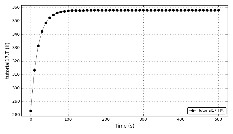
In this example we use the same heat transfer problem as in the tutorial 7.

The screenshot of the TCP/IP log server:

The temperature plot:

Files

Model report	tutorial17.xml
Runtime model report	tutorial17-rt.xml
Source code	tutorial17.py

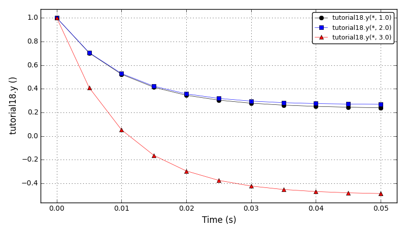
Tutorial 18

This tutorial shows one more problem solved using the NumPy arrays that operate on DAE Tools variables. The model is taken from the Sundials ARKODE (ark_analytic_sys.cpp). The ODE system is defined by the following system of equations:

dy/dt = A*y

where:

A = V * D * Vi
V = [1 -1 1; -1 2 1; 0 -1 2];
Vi = 0.25 * [5 1 -3; 2 2 -2; 1 1 1];
D = [-0.5 0 0; 0 -0.1 0; 0 0 lam];

lam is a large negative number.

The analytical solution to this problem is:

Y(t) = V*exp(D*t)*Vi*Y0

for t in the interval [0.0, 0.05], with initial condition y(0) = [1,1,1]’.

The stiffness of the problem is directly proportional to the value of “lamda”. The value of lamda should be negative to result in a well-posed ODE; for values with magnitude larger than 100 the problem becomes quite stiff.

In this example, we choose lamda = -100.

The solution:

lamda = -100
reltol = 1e-06
abstol = 1e-10

--------------------------------------
   t        y0        y1        y2
--------------------------------------
 0.0050   0.70327   0.70627   0.41004
 0.0100   0.52267   0.52865   0.05231
 0.0150   0.41249   0.42145  -0.16456
 0.0200   0.34504   0.35696  -0.29600
 0.0250   0.30349   0.31838  -0.37563
 0.0300   0.27767   0.29551  -0.42383
 0.0350   0.26138   0.28216  -0.45296
 0.0400   0.25088   0.27459  -0.47053
 0.0450   0.24389   0.27053  -0.48109
 0.0500   0.23903   0.26858  -0.48740
--------------------------------------

The plot of the ‘y0’, ‘y1’, ‘y2’ variables:

Files

Model report	tutorial18.xml
Runtime model report	tutorial18-rt.xml
Source code	tutorial18.py

Tutorial 19

This tutorial introduces the thermo physical property packages.

Since there are many thermo packages with a very different API the CapeOpen standard has been adopted in daetools. This way, all thermo packages implementing the CapeOpen thermo interfaces are automatically vailable to daetools. Those which do not are wrapped by the class with the CapeOpen conforming API. At the moment, two types of thermophysical property packages are implemented:

• Any CapeOpen v1.1 thermo package (available only in Windows)

• CoolProp thermo package (available for all platforms) wrapped in the class with the CapeOpen interface.

The central point is the daeThermoPhysicalPropertyPackage class. It can load any COM component that implements CapeOpen 1.1 ICapeThermoPropertyPackageManager interface or the CoolProp thermo package.

The framework provides low-level functions (specified in the CapeOpen standard) in the daeThermoPhysicalPropertyPackage class and the higher-level functions in the auxiliary daeThermoPackage class defined in the daetools/pyDAE/thermo_packages.py file. The low-level functions are defined in the ICapeThermoCoumpounds and ICapeThermoPropertyRoutine CapeOpen interfaces. These functions come in two flavours:

1. The ordinary functions return adouble/adouble_array objects and can only be used to specify equations:

   • GetCompoundConstant (from ICapeThermoCoumpounds interface)

   • GetTDependentProperty (from ICapeThermoCoumpounds interface)

   • GetPDependentProperty (from ICapeThermoCoumpounds interface)

   • CalcSinglePhaseScalarProperty (from ICapeThermoPropertyRoutine interface: scalar version)

   • CalcSinglePhaseVectorProperty (from ICapeThermoPropertyRoutine interface: vector version)

   • CalcTwoPhaseScalarProperty (from ICapeThermoPropertyRoutine interface: scalar version)

   • CalcTwoPhaseVectorProperty (from ICapeThermoPropertyRoutine interface: vector version)

2. The functions starting with the underscores can be used for calculations (they use and return float values):

   • _GetCompoundConstant

   • _GetTDependentProperty

   • _GetPDependentProperty

   • _CalcSinglePhaseScalarProperty

   • _CalcSinglePhaseVectorProperty

   • _CalcTwoPhaseScalarProperty

   • _CalcTwoPhaseVectorProperty

The daeThermoPackage auxiliary class offers functions to calculate specified properties, for instance:

• Transport properties:

  • cp, kappa, mu, Dab (heat capacity, thermal conductivity, dynamic viscosity, diffusion coefficient)

• Thermodynamic properties:

  • rho

  • h, s, G, H, I (enthalpy, entropy, gibbs/helmholtz/internal energy)

  • h_E, s_E, G_E, H_E, I_E, V_E (excess enthalpy, entropy, gibbs/helmholtz/internal energy, volume)

  • f and phi (fugacity and coefficient of fugacity)

  • a and gamma (activity and the coefficient of activity)

  • z (compressibility factor)

  • K, surfaceTension (ratio of fugacity coefficients and the surface tension)

Nota bene:

Some of the above functions return scalars while the others return arrays of values. Check the thermo_packages.py file for details.

All functions return properties in the SI units (as specified in the CapeOpen 1.1 standard).

Known issues:

• Many properties from the CapeOpen standard are not supported by all thermo packages.

• CalcEquilibrium from the ICapeThermoEquilibriumRoutine is not supported.

• CoolProp does not provide transport models for many compounds.

• The function calls are NOT thread safe.

• The code generation will NOT work for models using the thermo packages.

• Some CapeOpen thermo packags refuse to return properties for mass basis (i.e. density).

In this tutorial, we use a very simple model: a quantity of liquid (water + ethanol mixture) is heated using the constant input power. The model uses a thermo package to calculate the commonly used transport properties such as specific heat capacity, thermal conductivity, dynamic viscosity and binary diffusion coefficients. First, the low-level functions are tested for CapeOpen and CoolProp packages in the test_single_phase, test_two_phase, test_coolprop_single_phase functions. The results depend on the options selected in the CapeOpen package (equation of state, etc.). Then, the model that uses a thermo package is simulated.

The plot of the specific heat capacity as a function of temperature:

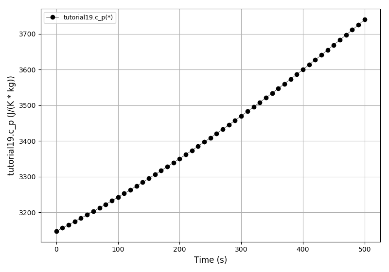
Nota bene:

There is a difference between results in Windows and other platforms since the CapeOpen thermo packages are available only in Windows.

Files

Model report	tutorial19.xml
Runtime model report	tutorial19-rt.xml
Source code	tutorial19.py

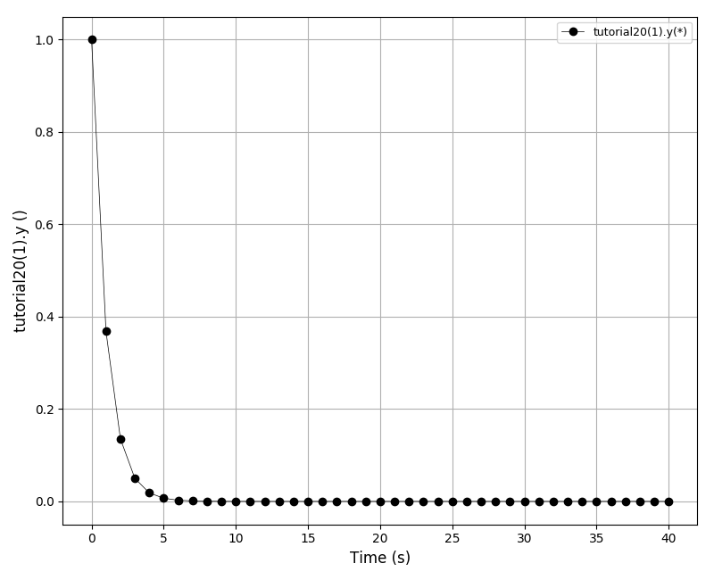
Tutorial 20

This tutorial illustrates the support variable constraints available in Sundials IDA solver. Benchmarks are available from Matlab documentation.

1. Absolute Value Function:

   dy/dt = -fabs(y)

   solved on the interval [0,40] with the initial condition y(0) = 1. The solution of this ODE decays to zero. If the solver produces a negative solution value, the computation eventually will fail as the calculated solution diverges to -inf. Using the constraint y >= 0 resolves this problem.

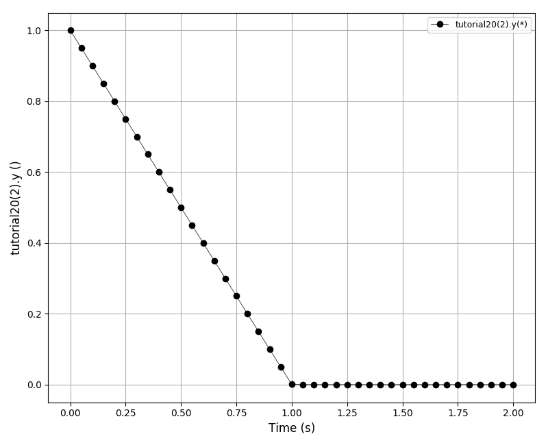
2. The Knee problem:

   epsilon * dy/dt = (1-t)*y - y**2

   solved on the interval [0,2] with the initial condition y(0) = 1. The parameter epsilon is 0 < epsilon << 1 and in this example equal to 1e-6. The solution follows the y = 1-x isocline for the whole interval of integration which is incorrect. Using the constraint y >= 0 resolves the problem.

In DAE Tools contraints follow the Sundials IDA solver implementation and can be specified using the valueConstraint argument of the daeVariableType class __init__ function:

• eNoConstraint (default)

• eValueGTEQ: imposes >= 0 constraint

• eValueLTEQ: imposes <= 0 constraint

• eValueGT: imposes > 0 constraint

• eValueLT: imposes < 0 constraint

and changed for individual variables using daeVariable.SetValueConstraint functions.

Absolute Value Function solution plot:

The Knee problem solution plot:

Files

Source code

tutorial20.py

Tutorial 21

This tutorial introduces different methods for evaluation of equations in parallel. Equations residuals, Jacobian matrix and sensitivity residuals can be evaluated in parallel using two methods

1. The Evaluation Tree approach (default)

   OpenMP API is used for evaluation in parallel. This method is specified by setting daetools.core.equations.evaluationMode option in daetools.cfg to “evaluationTree_OpenMP” or setting the simulation property:

   simulation.EvaluationMode = eEvaluationTree_OpenMP

   numThreads controls the number of OpenMP threads in a team. If numThreads is 0 the default number of threads is used (the number of cores in the system). Sequential evaluation is achieved by setting numThreads to 1.

2. The Compute Stack approach

   Equations can be evaluated in parallel using:

   1. OpenMP API for general purpose processors and manycore devices.

      This method is specified by setting daetools.core.equations.evaluationMode option in daetools.cfg to “computeStack_OpenMP” or setting the simulation property:

      simulation.EvaluationMode = eComputeStack_OpenMP

      numThreads controls the number of OpenMP threads in a team. If numThreads is 0 the default number of threads is used (the number of cores in the system). Sequential evaluation is achieved by setting numThreads to 1.

   2. OpenCL framework for streaming processors and heterogeneous systems.

      This type is implemented in an external Python module pyEvaluator_OpenCL. It is up to one order of magnitude faster than the Evaluation Tree approach. However, it does not support external functions nor thermo-physical packages.

      OpenCL evaluators can use a single or multiple OpenCL devices. It is required to install OpenCL drivers/runtime libraries. Intel: https://software.intel.com/en-us/articles/opencl-drivers AMD: https://support.amd.com/en-us/kb-articles/Pages/OpenCL2-Driver.aspx NVidia: https://developer.nvidia.com/opencl

Files

Source code

tutorial21.py

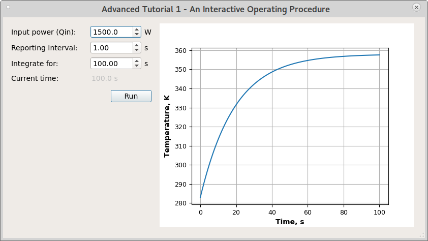
Advanced Tutorial 1

This tutorial presents a user-defined simulation which instead of simply integrating the system shows the pyQt graphical user interface (GUI) where the simulation can be manipulated (a sort of interactive operating procedure).

The model in this example is the same as in the tutorial 4.

The simulation.Run() function is modifed to show the graphical user interface (GUI) that allows to specify the input power of the heater (degree of freedom), a time period for integration, and a reporting interval. The GUI also contains the temperature plot updated in real time, as the simulation progresses.

The screenshot of the pyQt GUI:

Files

Model report	tutorial_adv_1.xml
Runtime model report	tutorial_adv_1-rt.xml
Source code	tutorial_adv_1.py

Advanced Tutorial 2

This tutorial demonstrates a solution of a discretized population balance using high resolution upwind schemes with flux limiter.

Reference: Qamar S., Elsner M.P., Angelov I.A., Warnecke G., Seidel-Morgenstern A. (2006) A comparative study of high resolution schemes for solving population balances in crystallization. Computers and Chemical Engineering 30(6-7):1119-1131. doi:10.1016/j.compchemeng.2006.02.012

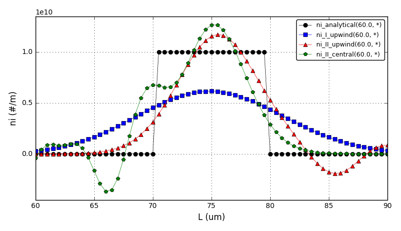
It shows a comparison between the analytical results and various discretization schemes:

• I order upwind scheme

• II order central scheme

• Cell centered finite volume method solved using the high resolution upwind scheme (Van Leer k-interpolation with k = 1/3 and Koren flux limiter)

The problem is from the section 3.1 Size-independent growth.

Could be also found in: Motz S., Mitrović A., Gilles E.-D. (2002) Comparison of numerical methods for the simulation of dispersed phase systems. Chemical Engineering Science 57(20):4329-4344. doi:10.1016/S0009-2509(02)00349-4

The comparison of number density functions between the analytical solution and the high-resolution scheme:

The comparison of number density functions between the analytical solution and the I order upwind, II order upwind and II order central difference schemes:

Files

Model report	tutorial_adv_2.xml
Runtime model report	tutorial_adv_2-rt.xml
Source code	tutorial_adv_2.py

Advanced Tutorial 3

This tutorial introduces the following concepts:

• DAE Tools code-generators

  • Modelica code-generator

  • gPROMS code-generator

  • FMI code-generator (for Co-Simulation)

• DAE Tools model-exchange capabilities:

  • Scilab/GNU_Octave/Matlab MEX functions

  • Simulink S-functions

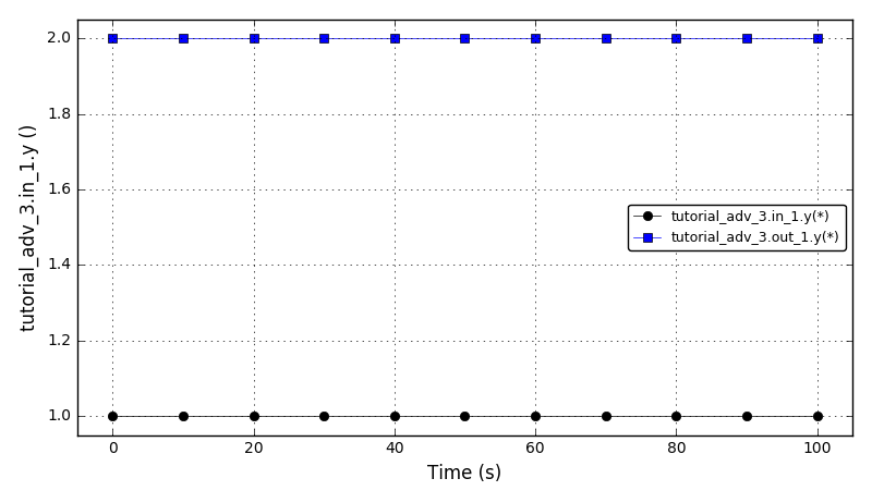
The model represent a simple multiplier block. It contains two inlet and two outlet ports. The outlets values are equal to inputs values multiplied by a multiplier “m”:

out1.y   = m1   x in1.y
out2.y[] = m2[] x in2.y[]

where multipliers m1 and m2[] are:

STN Multipliers
   case variableMultipliers:
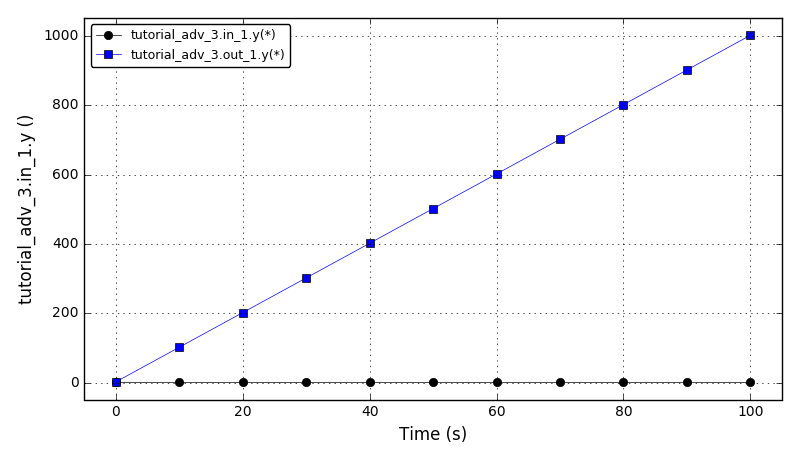
      dm1/dt   = p1
      dm2[]/dt = p2
   case constantMultipliers:
      dm1/dt   = 0
      dm2[]/dt = 0

(that is the multipliers can be constant or variable).

The ports in1 and out1 are scalar (width = 1). The ports in2 and out2 are vectors (width = 1).

Achtung, Achtung!! Notate bene:

1. Inlet ports must be DOFs (that is to have their values asssigned), for they can’t be connected when the model is simulated outside of daetools context.

2. Only scalar output ports are supported at the moment!! (Simulink issue)

The plot of the inlet ‘y’ variable and the multiplied outlet ‘y’ variable for the constant multipliers (m1 = 2):

The plot of the inlet ‘y’ variable and the multiplied outlet ‘y’ variable for the variable multipliers (dm1/dt = 10, m1(t=0) = 2):

Files

Model report	tutorial_adv_3.xml
Runtime model report	tutorial_adv_3-rt.xml
Source code	tutorial_adv_3.py

Advanced Tutorial 4

This tutorial illustrates the OpenCS code generator. For the given DAE Tools simulation it generates input files for OpenCS simulation, either for a single CPU or for a parallel simulation using MPI. The model is identical to the model in the tutorial 11.

The OpenCS framework currently does not support:

• Discontinuous equations (STNs and IFs)

• External functions

• Thermo-physical property packages

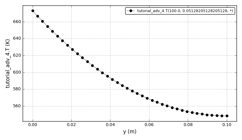
The temperature plot (at t=100s, x=0.5128, y=*):

Files

Model report	tutorial_adv_4.xml
Runtime model report	tutorial_adv_4-rt.xml
Source code	tutorial_adv_4.py

Code Verification Test 1

Code verification using the Method of Exact Solutions.

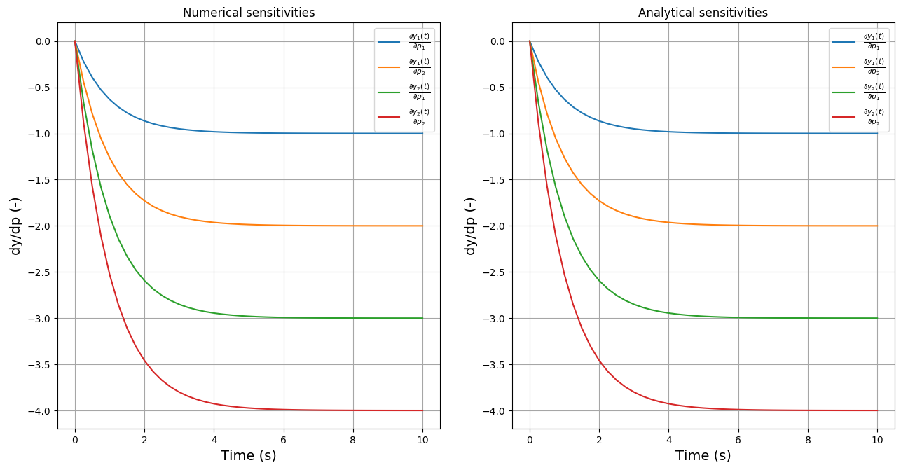
Here, the numerical solution and numerical sensitivities for the Constant coefficient first order equations are compared to the available analytical solution.

The sensitivity analysis is enabled and the sensitivities are reported to the data reporter. The sensitivity data can be obtained in two ways:

• Directly from the DAE solver in the user-defined Run function using the DAESolver.SensitivityMatrix property.

• From the data reporter as any ordinary variable.

The comparison between the numerical and the analytical sensitivities:

Files

Model report	tutorial_cv_1.xml
Runtime model report	tutorial_cv_1-rt.xml
Source code	tutorial_cv_1.py

Code Verification Test 2

Code verification using the Method of Manufactured Solutions.

References:

1. G. Tryggvason. Method of Manufactured Solutions, Lecture 33: Predictivity-I, 2011. PDF

2. K. Salari and P. Knupp. Code Verification by the Method of Manufactured Solutions. SAND2000 – 1444 (2000). doi:10.2172/759450

3. P.J. Roache. Fundamentals of Verification and Validation. Hermosa, 2009. ISBN-10:0913478121

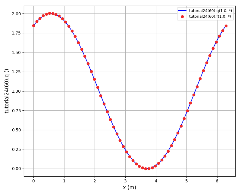
The procedure for the transient convection-diffusion (Burger’s) equation:

L(f) = df/dt + f*df/dx - D*d2f/dx2 = 0

is the following:

1. Pick a function (q, the manufactured solution):

   q = A + sin(x + Ct)
   

2. Compute the new source term (g) for the original problem:

   g = dq/dt + q*dq/dx - D*d2q/dx2
   

3. Solve the original problem with the new source term:

   df/dt + f*df/dx - D*d2f/dx2 = g
   

Since L(f) = g and g = L(q), consequently we have: f = q. Therefore, the computed numerical solution (f) should be equal to the manufactured one (q).

The terms in the source g term are:

dq/dt   = C * cos(x + C*t)
dq/dx   = cos(x + C*t)
d2q/dx2 = -sin(x + C*t)

The equations are solved for Dirichlet boundary conditions:

f(x=0)   = q(x=0)   = A + sin(0 + Ct)
f(x=2pi) = q(x=2pi) = A + sin(2pi + Ct)

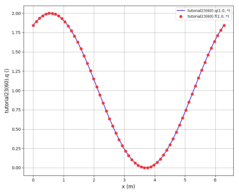
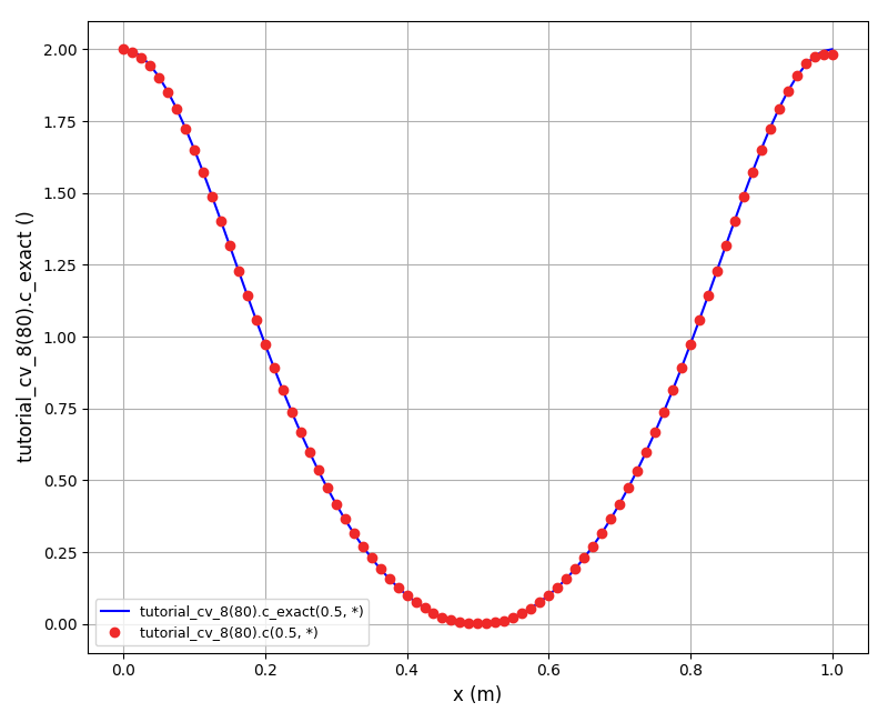
Numerical vs. manufactured solution plot (no. elements = 60, t = 1.0s):

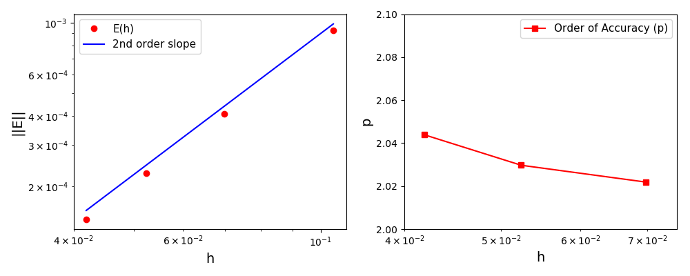
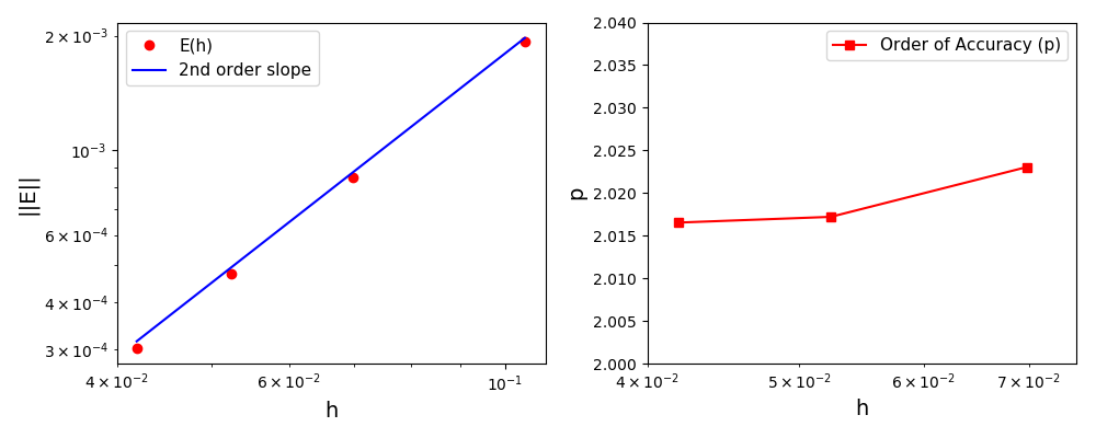
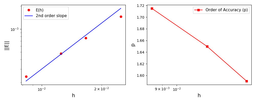
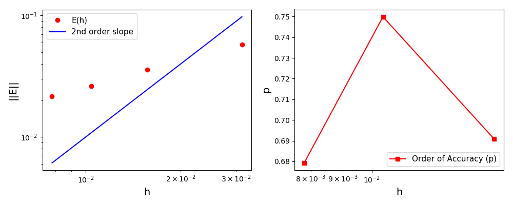
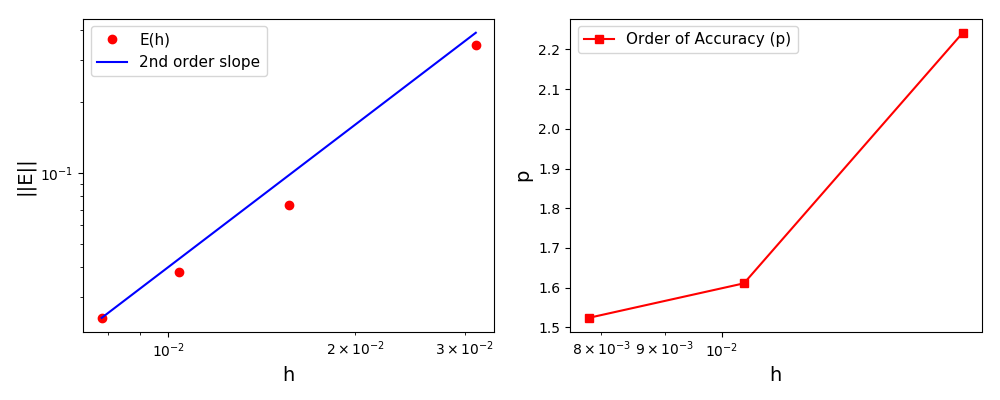
The normalised global errors and the order of accuracy plots (no. elements = [60, 90, 120, 150], t = 1.0s):

Files

Model report	tutorial_cv_2.xml
Runtime model report	tutorial_cv_2-rt.xml
Source code	tutorial_cv_2.py

Code Verification Test 3

Code verification using the Method of Manufactured Solutions.

References:

1. G. Tryggvason. Method of Manufactured Solutions, Lecture 33: Predictivity-I, 2011. PDF

2. K. Salari and P. Knupp. Code Verification by the Method of Manufactured Solutions. SAND2000 – 1444 (2000). doi:10.2172/759450

3. P.J. Roache. Fundamentals of Verification and Validation. Hermosa, 2009. ISBN-10:0913478121

The problem in this tutorial is identical to tutorial_cv_3. The only difference is that the Neumann boundary conditions are applied:

df(x=0)/dx   = dq(x=0)/dx   = cos(0 + Ct)
df(x=2pi)/dx = dq(x=2pi)/dx = cos(2pi + Ct)

Numerical vs. manufactured solution plot (no. elements = 60, t = 1.0s):

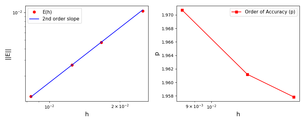
The normalised global errors and the order of accuracy plots (no. elements = [60, 90, 120, 150], t = 1.0s):

Files

Model report	tutorial_cv_3.xml
Runtime model report	tutorial_cv_3-rt.xml
Source code	tutorial_cv_3.py

Code Verification Test 4

Code verification using the Method of Manufactured Solutions.

Reference:

1. K. Salari and P. Knupp. Code Verification by the Method of Manufactured Solutions. SAND2000 – 1444 (2000). doi:10.2172/759450

The problem in this tutorial is the transient convection-diffusion equation distributed on a rectangular 2D domain with u and v components of velocity:

L(u) = du/dt + (d(uu)/dx + d(uv)/dy) - ni * (d2u/dx2 + d2u/dy2) = 0
L(v) = dv/dt + (d(vu)/dx + d(vv)/dy) - ni * (d2v/dx2 + d2v/dy2) = 0

The manufactured solutions are:

um = u0 * (sin(x**2 + y**2 + w0*t) + eps)
vm = v0 * (cos(x**2 + y**2 + w0*t) + eps)

The terms in the new sources Su and Sv are computed using the daetools derivative functions (dt, d and d2).

Again, the Dirichlet boundary conditions are used:

u(LB, y)  = um(LB, y)
u(UB, y)  = um(UB, y)
u(x,  LB) = um(x,  LB)
u(x,  UB) = um(x,  UB)

v(LB, y)  = vm(LB, y)
v(UB, y)  = vm(UB, y)
v(x,  LB) = vm(x,  LB)
v(x,  UB) = vm(x,  UB)

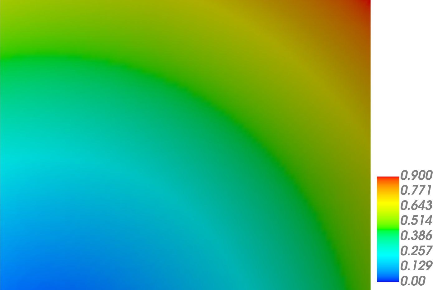
Steady-state results (w0 = 0.0) for the u-component:

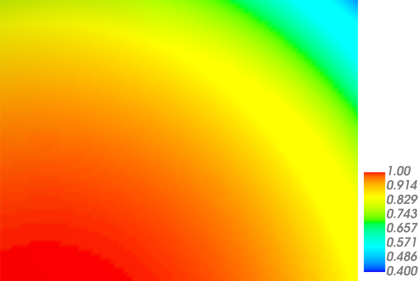
Steady-state results (w0 = 0.0) for the v-component:

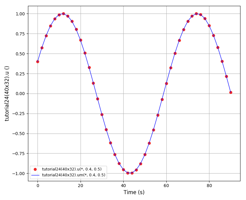
Numerical vs. manufactured solution plot (u velocity component, 40x32 grid):

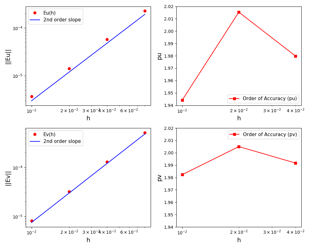
The normalised global errors and the order of accuracy plots (grids 10x8, 20x16, 40x32, 80x64):

Files

Model report	tutorial_cv_4.xml
Runtime model report	tutorial_cv_4-rt.xml
Source code	tutorial_cv_4.py

Code Verification Test 5

Code verification using the Method of Manufactured Solutions.

This problem and its solution in COMSOL Multiphysics software is described in the COMSOL blog: Verify Simulations with the Method of Manufactured Solutions (2015).

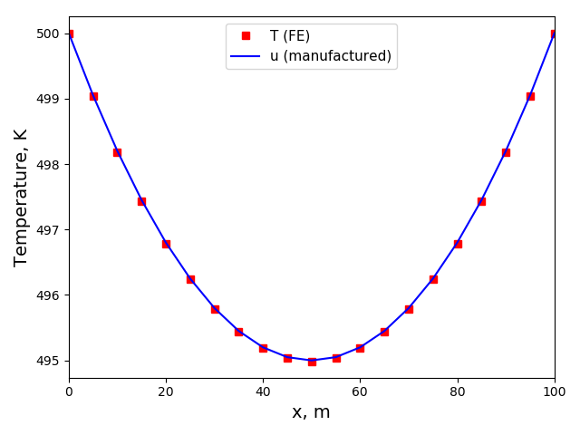
Here, a 1D transient heat conduction problem in a bar of length L is solved using the FE method:

dT/dt - k/(rho*cp) * d2T/dx2 = 0, x in [0,L]

with the following boundary:

T(0,t) = 500 K
T(L,t) = 500 K

and initial conditions:

T(x,0) = 500 K

The manufactured solution is given by function u(x):

u(x) = 500 + (x/L) * (x/L - 1) * (t/tau)

The new source term is:

g(x) = du/dt - k/(rho*cp) * d2u/dx2

The terms in the source g term are:

du_dt   = (x/L) * (x/L - 1) * (1/tau)
d2u_dx2 = (2/(L**2)) * (t/tau)

Finally, the original problem with the new source term is:

dT/dt - k/(rho*cp) * d2T/dx2 = g(x), x in [0,L]

The mesh is linear (a bar) with a length of 100 m:

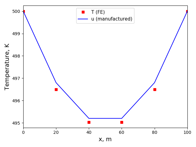
The comparison plots for the coarse mesh and linear elements:

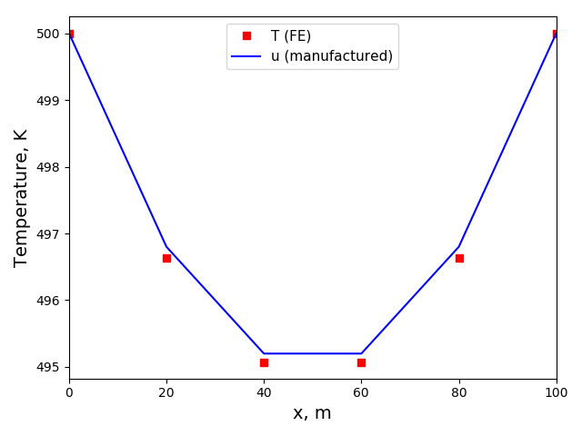
The comparison plots for the coarse mesh and quadratic elements:

The comparison plots for the fine mesh and linear elements:

The comparison plots for the fine mesh and quadratic elements:

Files

Model report	tutorial_cv_5.xml
Runtime model report	tutorial_cv_5-rt.xml
Source code	tutorial_cv_5.py

Code Verification Test 6

Code verification using the Method of Exact Solutions.

Reference (section 3.3):

• B. Koren. A robust upwind discretization method for advection, diffusion and source terms. Department of Numerical Mathematics. Report NM-R9308 (1993). PDF

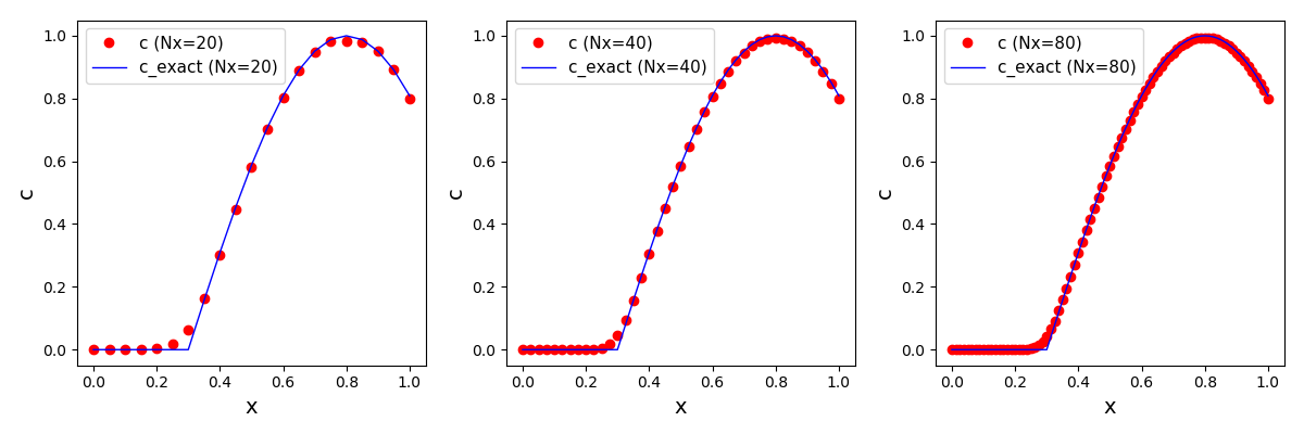
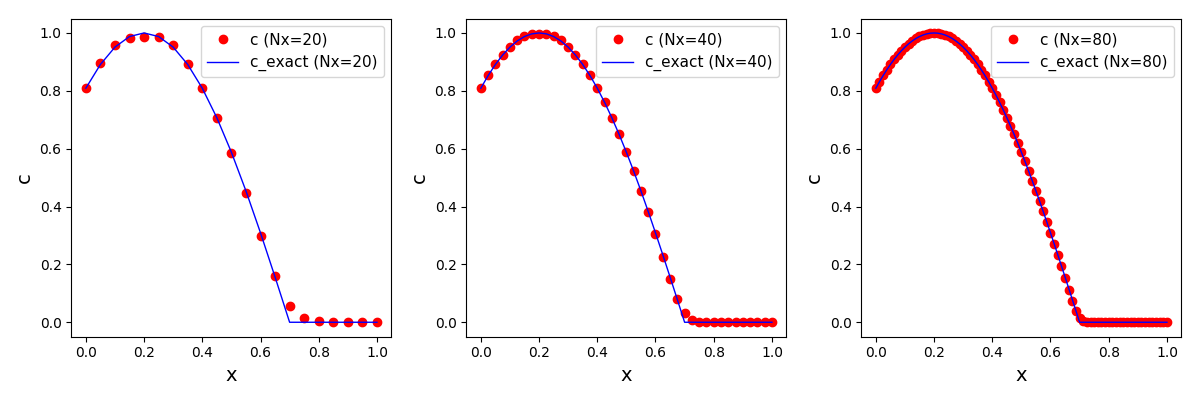
The problem in this tutorial is 1D transient convection-diffusion equation:

dc_dt + u*dc/dx - D*d2c/dc2 = 0

The equation is solved using the high resolution cell-centered finite volume upwind scheme with flux limiter described in the article.

Numerical vs. exact solution plots (Nx = [20, 40, 80]):

Files

Model report	tutorial_cv_6.xml
Runtime model report	tutorial_cv_6-rt.xml
Source code	tutorial_cv_6.py

Code Verification Test 7

Code verification using the Method of Manufactured Solutions.

Reference (section 4.2):

• B. Koren. A robust upwind discretization method for advection, diffusion and source terms. Department of Numerical Mathematics. Report NM-R9308 (1993). PDF

The problem in this tutorial is 1D steady-state convection-diffusion (Burger’s) equation:

u*dc/dx - D*d2c/dc2 = 0

The manufactured solution is:

c(x) = 0.5 * (1 - cos(2*pi*(x-a)/(b-a))), x in [a,b]
c(x) = 0, otherwise

The new source term is:

s(x) = pi/(b-a) * u * sin(2*pi*(x-a)/(b-a)) - 2*(pi/(b-a))**2 * D * cos(2*pi*(x-a)/(b-a)), x in [a,b]
s(x) = 0, otherwise

The modified equation:

u*dc/dx - D*d2c/dc2 = s(x)

is solved using the high resolution cell-centered finite volume upwind scheme with flux limiter described in the article.

In order to obtain the consistent discretisation of the convection and the source terms an integral of the source term: S(x) = 1/u * Integral s(x)*dx must be calculated. The result of integration is given as:

S(x) = 0.5 * (1 - cos(2*pi*(x-a)/(b-a)))) - pi/(b-a) * D/u * sin(2*pi*(x-a)/(b-a))), x in [a,b]
S(x) = 0, otherwise

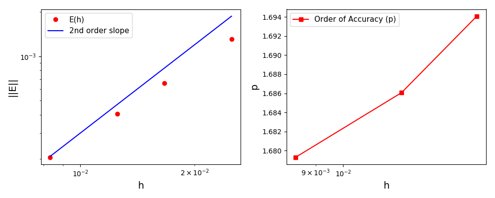
Numerical vs. manufactured solution plot (Nx=80):

The normalised global errors and the order of accuracy plots for the Koren flux limiter (grids 40, 60, 80, 120):

The normalised global errors and the order of accuracy plots for the Superbee flux limiter (grids 40, 60, 80, 120):

Files

Model report	tutorial_cv_7.xml
Runtime model report	tutorial_cv_7-rt.xml
Source code	tutorial_cv_7.py

Code Verification Test 8

Code verification using the Method of Manufactured Solutions.

Reference (page 64):

• W. Hundsdorfer. Numerical Solution of Advection-Diffusion-Reaction Equations. Lecture notes (2000), Thomas Stieltjes Institute. PDF

The problem in this tutorial is 1D transient convection-reaction equation:

dc/dt + dc/dx = c**2

The exact solution is:

c(x,t) = sin(pi*(x-t))**2 / (1 - t*sin(pi*(x-t))**2)

The equation is solved using the high resolution cell-centered finite volume upwind scheme with flux limiter described in the article. The boundary and initial conditions are obtained from the exact solution.

The consistent discretisation of the convection and the source terms cannot be done since the constant C1 in the integral of the source term:

S(x) = 1/u * Integral s(x)*dx = u**/3 + C1 

is not known. Therefore, the numerical cell average is used:

Snum(x) = Integral s(x)*dx = s(i) * (x[i]-x[i-1]).

Numerical vs. manufactured solution plot (Nx=80):

The normalised global errors and the order of accuracy plots for the Koren flux limiter (grids 40, 60, 80, 120):

Files

Model report	tutorial_cv_8.xml
Runtime model report	tutorial_cv_8-rt.xml
Source code	tutorial_cv_8.py

Code Verification Test 9

Code verification using the Method of Exact Solutions (Solid Body Rotation problem).

Reference (section 4.4.6.1 Solid Body Rotation):

• D. Kuzmin (2010). A Guide to Numerical Methods for Transport Equations. PDF

Solid body rotation illustrates the ability of a numerical scheme to transport initial data without distortion. Here, a 2D transient convection problem in a rectangular (0,1)x(0,1) domain is solved using the FE method:

dc/dt + div(u*c) = 0, in Omega = (0,1)x(0,1)

The initial conditions define a conical body which is rotated counterclockwise around the point (0.5, 0.5) using the velocity field u = (0.5 - y, x - 0.5). The cone is defined by the following equation:

r0 = 0.15
(x0, y0) = (0.5, 0.25)
c(x,y,0) = 1 - (1/r0) * sqrt((x-x0)**2 + (y-y0)**2)

After t = 2pi the body should arrive at the starting position.

Homogeneous Dirichlet boundary conditions are prescribed at all four edges:

c(x,y,t) = 0.0

The mesh is a square (0,1)x(0,1):

The solution plot at t = 0 and t = 2pi (96x96 grid):

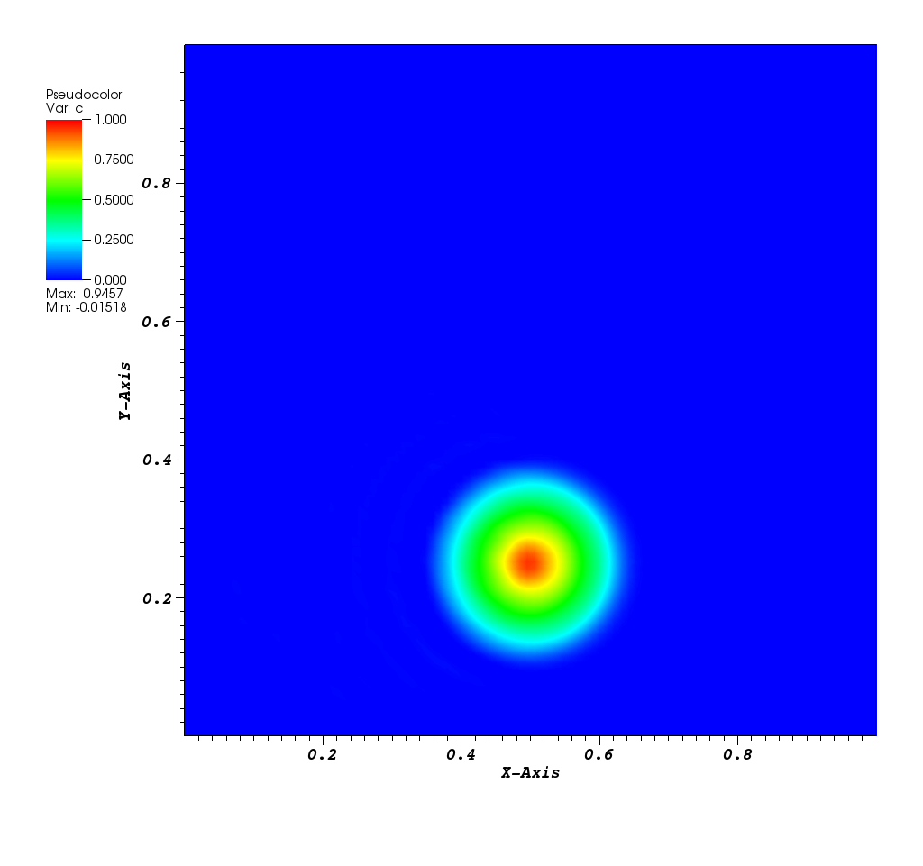
Animations for 32x32 and 96x96 grids:

It can be observed that the shape of the cone is preserved. Also, since the above equation is hyperbolic some oscillations in the solution out of the cone appear, which are more pronounced for coarser grids. This problem was resolved in the original example using the flux linearisation technique.

The normalised global errors and the order of accuracy plots (no. elements = [32x32, 64x64, 96x96, 128x128], t = 2pi):

Files

Model report	tutorial_cv_9.xml
Runtime model report	tutorial_cv_9-rt.xml
Source code	tutorial_cv_9.py

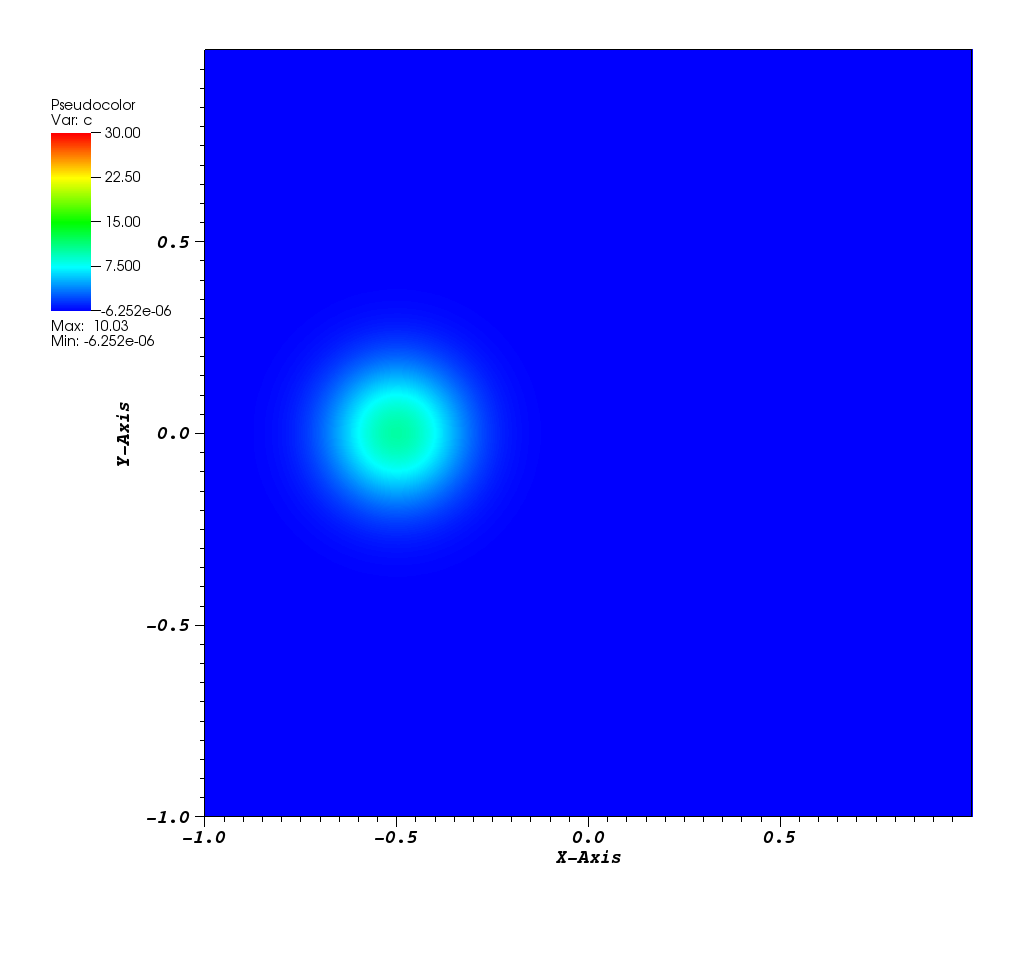
Code Verification Test 10

Code verification using the Method of Exact Solutions (Rotating Gaussian Hill problem).

Reference (section 4.4.6.3 Convection-Diffusion):

• D. Kuzmin (2010). A Guide to Numerical Methods for Transport Equations. PDF

Here, a 2D transient convection-diffusion problem in a rectangular (-1,1)x(-1,1) domain is solved using the FE method:

dc/dt + div(u*c) - eps*nabla(c) = 0, in Omega = (-1,1)x(-1,1)

The exact solution is given by the following function:

(x0, y0) = (0.0, 0.5)
x_bar(t) = x0*cos(t) - y0*sin(t)
y_bar(t) = -x0*sin(t) + y0*cos(t)
r2(x,y,t) = (x-x_bar(t))**2 + (y-y_bar(t))**2

c_exact(x,y,t) = 1.0 / (4*pi*eps*t) * exp(-r2(x,y,t) / (4*eps*t))

The initial conditions define a Gaussian hill which is rotated counterclockwise around the point (0.0, 0.0) using the velocity field u = (-y, x). Since at t = 0 the value of c_exact is the Dirac delta function it is better to start the simulation at t > 0. Therefore, the simulation is started and t = pi/2 by reinitialising variable c to:

c(x,y,pi/2) = c_exact(x,y,pi/2)

At t = 5/2 pi the peak smeared by the diffusion should arrive at the starting position.

Homogeneous Dirichlet boundary conditions are prescribed at all four edges:

c(x,y,t) = 0.0

The mesh is a rectangle (-1,1)x(-1,1):

The solution plots at t = pi/2 (the initial peak) and t = 5/2pi (96x96 grid):

Animations for 32x32 and 96x96 grids:

Again, some low-magnitude oscillations in the solution appear, which are more pronounced for coarser grids. In the original example this problem was resolved using the flux linearisation technique.

The normalised global errors and the order of accuracy plots (no. elements = [32x32, 64x64, 96x96, 128x128], t = 5/2pi):

Files

Model report	tutorial_cv_10.xml
Runtime model report	tutorial_cv_10-rt.xml
Source code	tutorial_cv_10.py

Code Verification Test 11

Code verification using the Method of Exact Solutions.

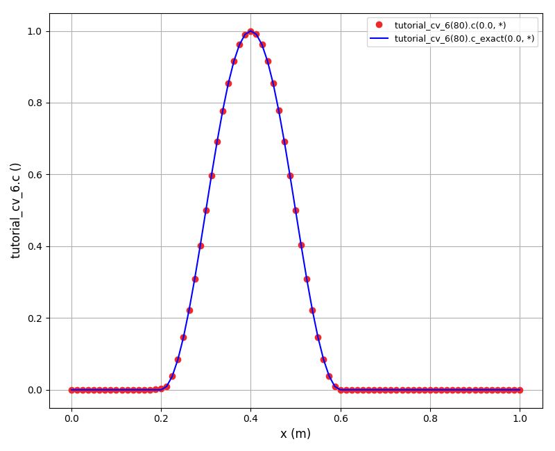
The problem is identical to the problem in the tutorial_cv_6. The only difference is that the flow is reversed to test the high resolution scheme for the reversed flow mode.

Numerical vs. exact solution plots (Nx = [20, 40, 80]):

Files

Model report	tutorial_cv_11.xml
Runtime model report	tutorial_cv_11-rt.xml
Source code	tutorial_cv_11.py

Tutorial deal.II 1

An introductory example of the support for Finite Elements in daetools. The basic idea is to use an external library to perform all low-level tasks such as management of mesh elements, degrees of freedom, matrix assembly, management of boundary conditions etc. deal.II library (www.dealii.org) is employed for these tasks. The mass and stiffness matrices and the load vector assembled in deal.II library are used to generate a set of algebraic/differential equations in the following form: [Mij]{dx/dt} + [Aij]{x} = {Fi}. Specification of additional equations such as surface/volume integrals are also available. The numerical solution of the resulting ODA/DAE system is performed in daetools together with the rest of the model equations.

The unique feature of this approach is a capability to use daetools variables to specify boundary conditions, time varying coefficients and non-linear terms, and evaluate quantities such as surface/volume integrals. This way, the finite element model is fully integrated with the rest of the model and multiple FE systems can be created and coupled together. In addition, non-linear and DAE finite element systems are automatically supported.

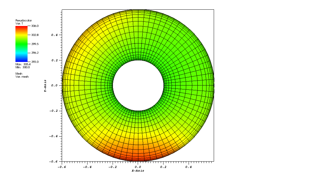
In this tutorial the simple transient heat conduction problem is solved using the finite element method:

dT/dt - kappa/(rho*cp)*nabla^2(T) = g(T) in Omega

The mesh is rectangular with two holes, similar to the mesh in step-49 deal.II example:

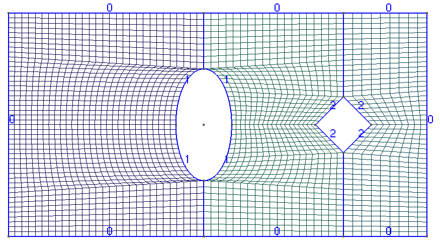
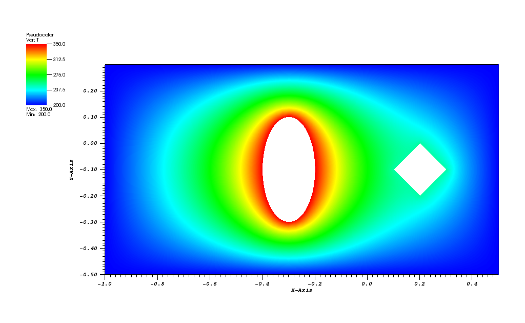
Dirichlet boundary conditions are set to 300 K on the outer rectangle, 350 K on the inner ellipse and 250 K on the inner diamond.

The temperature plot at t = 500s (generated in VisIt):

Animation:

Files

Model report	tutorial_dealii_1.xml
Runtime model report	tutorial_dealii_1-rt.xml
Source code	tutorial_dealii_1.py

Tutorial deal.II 2

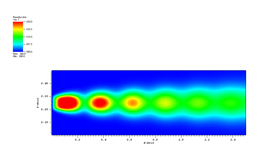
In this example a simple transient heat convection-diffusion equation is solved.

dT/dt - kappa/(rho*cp)*nabla^2(T) + nabla.(uT) = g(T) in Omega

The fluid flows from the left side to the right with constant velocity of 0.01 m/s. The inlet temperature for 0.2 <= y <= 0.3 is iven by the following expression:

T_left = T_base + T_offset*|sin(pi*t/25)| on dOmega

creating a bubble-like regions of higher temperature that flow towards the right end and slowly diffuse into the bulk flow of the fluid due to the heat conduction.

The mesh is rectangular with the refined elements close to the left/right ends:

The temperature plot at t = 500s:

Animation:

Files

Model report	tutorial_dealii_2.xml
Runtime model report	tutorial_dealii_2-rt.xml
Source code	tutorial_dealii_2.py

Tutorial deal.II 3

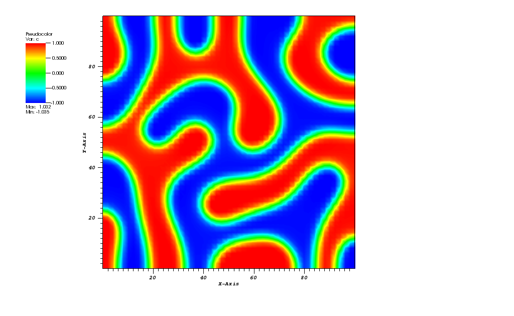
In this example the Cahn-Hilliard equation is solved using the finite element method. This equation describes the process of phase separation, where two components of a binary mixture separate and form domains pure in each component.

dc/dt - D*nabla^2(mu) = 0, in Omega
mu = c^3 - c - gamma*nabla^2(c)

The mesh is a simple square (0-100)x(0-100):

The concentration plot at t = 500s:

Animation:

Files

Model report	tutorial_dealii_3.xml
Runtime model report	tutorial_dealii_3-rt.xml
Source code	tutorial_dealii_3.py

Tutorial deal.II 4

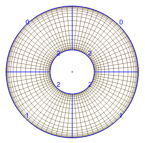
In this tutorial the transient heat conduction problem is solved using the finite element method:

dT/dt - kappa * nabla^2(Τ) = g in Omega

The mesh is a pipe submerged into water receiving the heat of the sun at the 45 degrees from the top-left direction, the heat from the suroundings and having the constant temperature of the inner tube. The boundary conditions are thus:

• [at boundary ID=0] Sun shine at 45 degrees, gradient heat flux = 2 kW/m**2 in direction n = (1,-1)

• [at boundary ID=1] Outer surface where y <= -0.5, constant flux of 2 kW/m**2

• [at boundary ID=2] Inner tube: constant temperature of 300 K

The pipe mesh is given below:

The temperature plot at t = 3600s:

Animation:

Files

Model report	tutorial_dealii_4.xml
Runtime model report	tutorial_dealii_4-rt.xml
Source code	tutorial_dealii_4.py

Tutorial deal.II 5

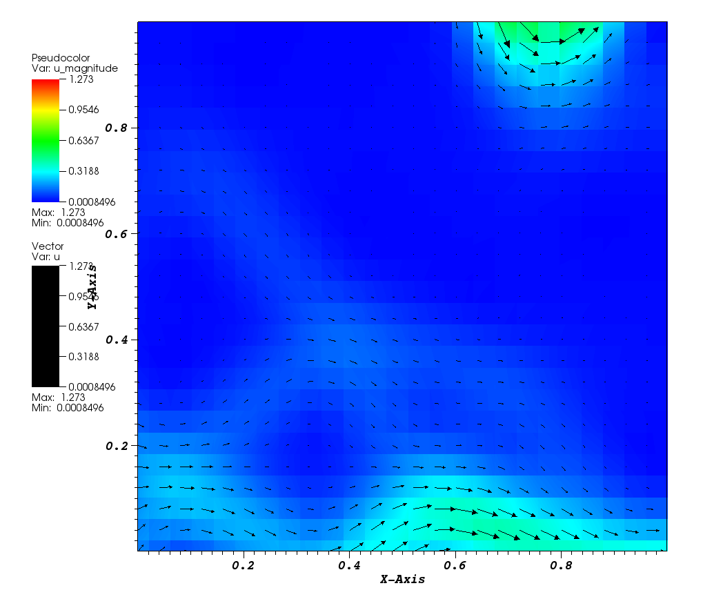
In this example a simple flow through porous media is solved (deal.II step-20).

K^{-1} u + nabla(p) = 0 in Omega
-div(u) = -f in Omega
p = g on dOmega

The mesh is a simple square:

The velocity magnitude plot:

Files

Model report	tutorial_dealii_5.xml
Runtime model report	tutorial_dealii_5-rt.xml
Source code	tutorial_dealii_5.py

Tutorial deal.II 6

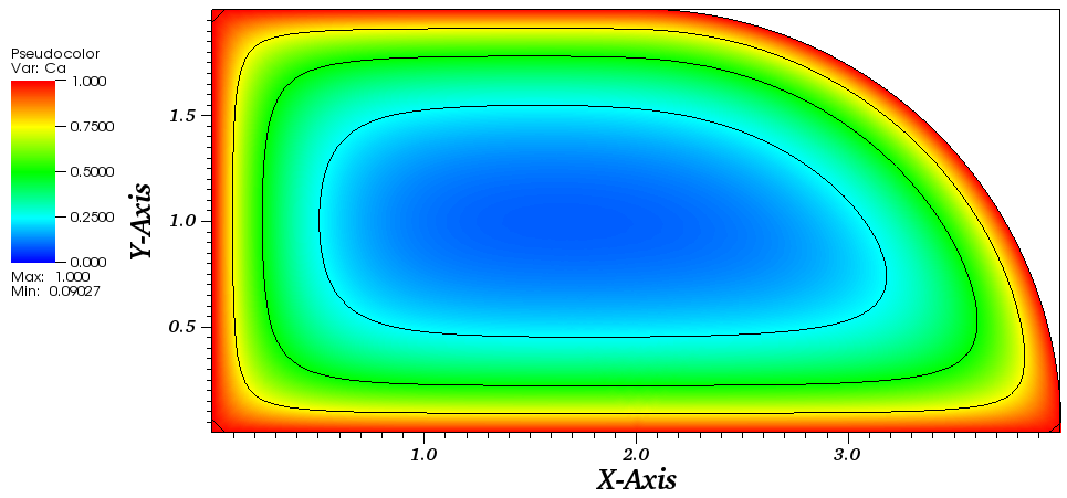
A simple steady-state diffusion and first-order reaction in an irregular catalyst shape (Proc. 6th Int. Conf. on Mathematical Modelling, Math. Comput. Modelling, Vol. 11, 375-319, 1988) applying Dirichlet and Robin type of boundary conditions.

D_eA * nabla^2(C_A) - k_r * C_A = 0 in Omega
D_eA * nabla(C_A) = k_m * (C_A - C_Ab) on dOmega1
C_A = C_Ab on dOmega2

The catalyst pellet mesh:

The concentration plot:

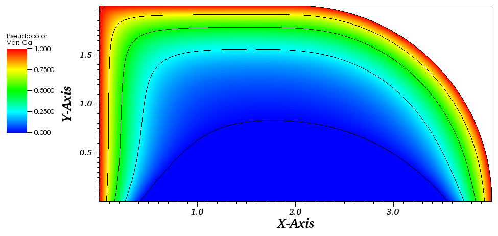
The concentration plot for Ca=Cab on all boundaries:

Files

Model report	tutorial_dealii_6.xml
Runtime model report	tutorial_dealii_6-rt.xml
Source code	tutorial_dealii_6.py

Tutorial deal.II 7

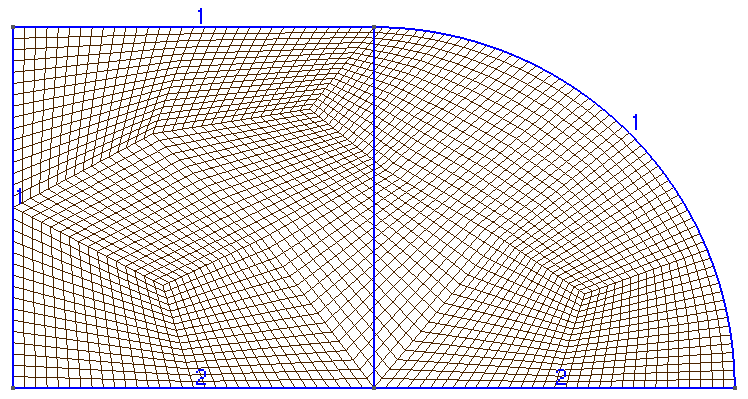
In this example 2D transient Stokes flow driven by the differences in buoyancy caused by the temperature differences in the fluid is solved (deal.II step-31).

The differences to the original problem are that the grid is not adaptive and no stabilisation method is used.

The problem can be described using the Stokes equations:

-div(2 * eta * eps(u)) + nabla(p) = -rho * beta * g * T in Omega
-div(u) = 0 in Omega
dT/dt + div(u * T) - div(k * nabla(T)) = gamma in Omega

The mesh is a simple square (0,1)x(0,1):

The temperature and the velocity vectors plot:

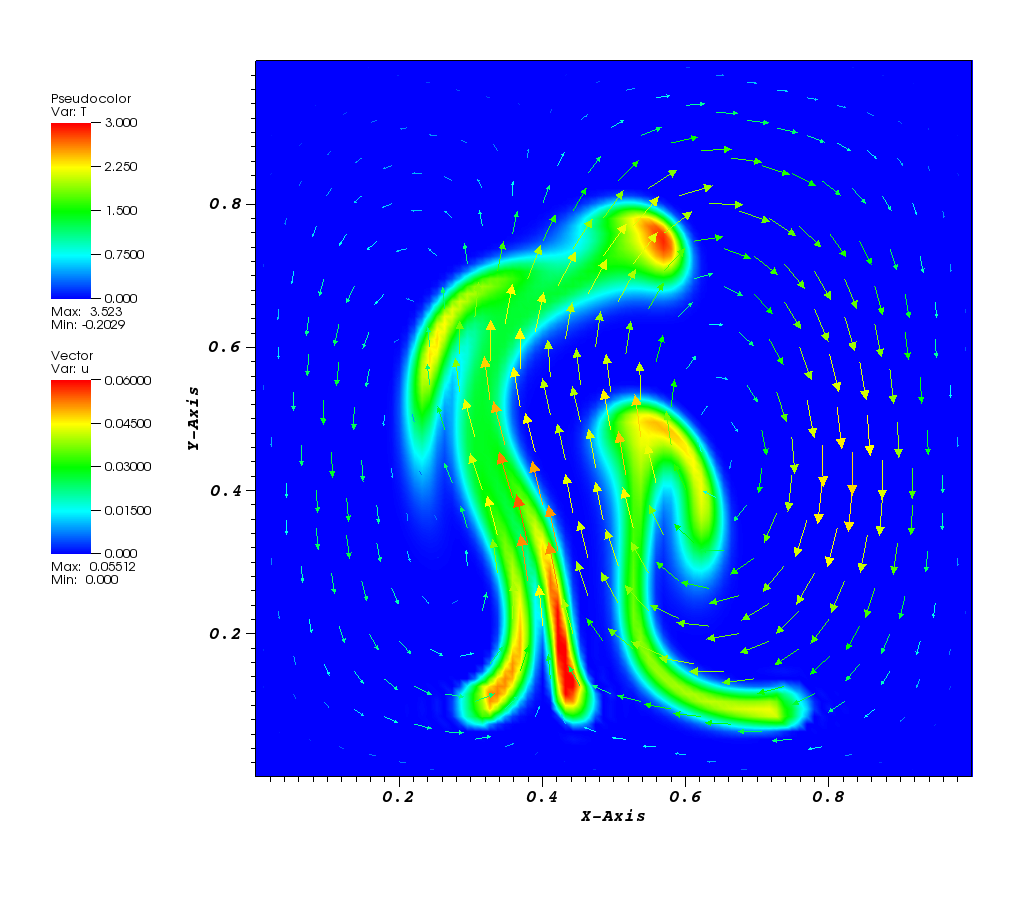
Animation:

Files

Model report	tutorial_dealii_7.xml
Runtime model report	tutorial_dealii_7-rt.xml
Source code	tutorial_dealii_7.py

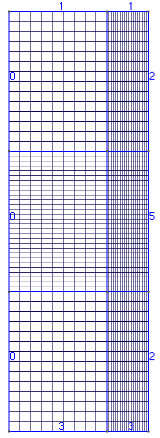
Tutorial deal.II 8

In this example a small parallel-plate reactor with an active surface is modelled.

This problem and its solution in COMSOL Multiphysics software is described in the Application Gallery: Transport and Adsorption (id=5).

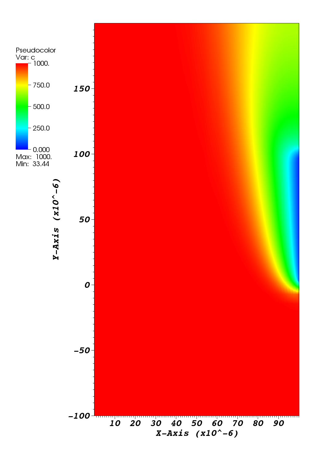
The transport in the bulk of the reactor is described by a convection-diffusion equation:

dc/dt - D*nabla^2(c) + div(uc) = 0 in Omega

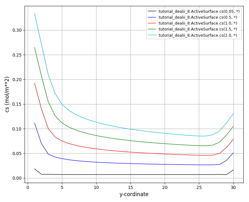
The material balance for the surface, including surface diffusion and the reaction rate is:

dc_s/dt - Ds*nabla^2(c_s) = -k_ads * c * (Gamma_s - c_s) + k_des * c_s in Omega_s

For the bulk, the boundary condition at the active surface couples the rate of the reaction at the surface with the flux of the reacting species and the concentration of the adsorbed species and bulk species:

n⋅(-D*nabla(c) + c*u) = -k_ads*c*(Gamma_s - c_s) + k_des*c_s

The boundary conditions for the surface species are insulating conditions.

The problem is modelled using two coupled Finite Element systems: 2D for bulk flow and 1D for the active surface. The linear interpolation is used to determine the bulk flow and active surface concentrations at the interface.

The mesh is rectangular with the refined elements close to the left/right ends:

The cs plot at t = 2s:

The c plot at t = 2s:

Animation:

Files

Model report	tutorial_dealii_8.xml
Runtime model report	tutorial_dealii_8-rt.xml
Source code	tutorial_dealii_8.py

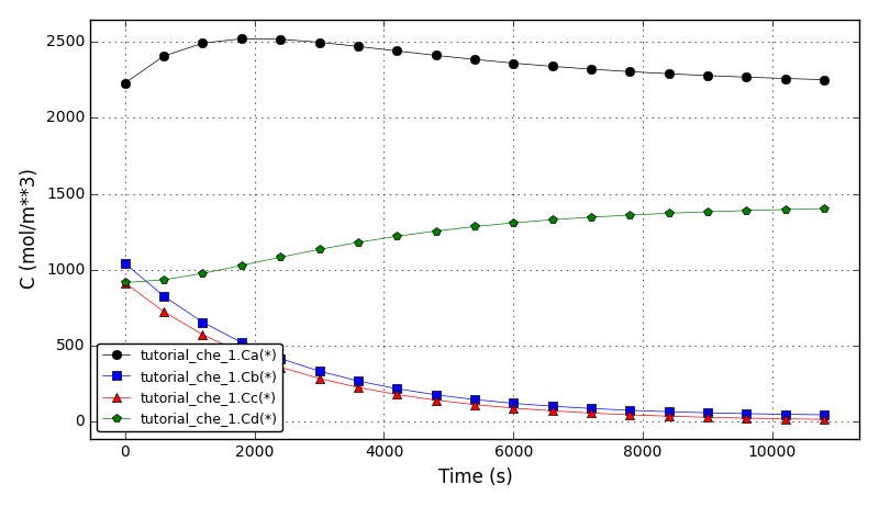
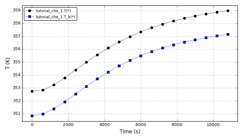
Chem. Eng. Example 1

Continuously Stirred Tank Reactor with energy balance and Van de Vusse reactions:

 A -> B -> C
2A -> D

Reference: G.A. Ridlehoover, R.C. Seagrave. Optimization of Van de Vusse Reaction Kinetics Using Semibatch Reactor Operation, Ind. Eng. Chem. Fundamen. 1973;12(4):444-447. doi:10.1021/i160048a700

The concentrations plot:

The temperatures plot:

Files

Model report	tutorial_che_1.xml
Runtime model report	tutorial_che_1-rt.xml
Source code	tutorial_che_1.py

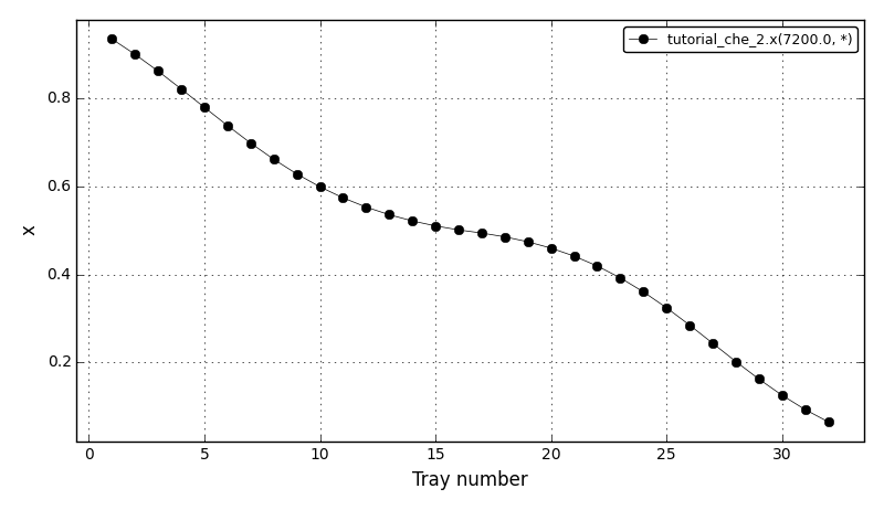
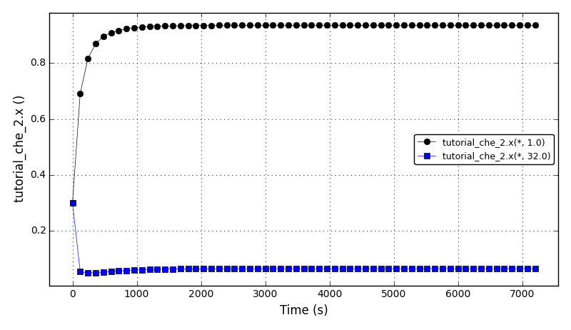
Chem. Eng. Example 2

Binary distillation column model.

Reference: J. Hahn, T.F. Edgar. An improved method for nonlinear model reduction using balancing of empirical gramians. Computers and Chemical Engineering 2002; 26:1379-1397. doi:10.1016/S0098-1354(02)00120-5

The liquid fraction after 120 min (x(reboiler)=0.935420, x(condenser)=0.064581):

The liquid fraction in the reboiler (tray 1) and in the condenser (tray 32):

Files

Model report	tutorial_che_2.xml
Runtime model report	tutorial_che_2-rt.xml
Source code	tutorial_che_2.py

Chem. Eng. Example 3

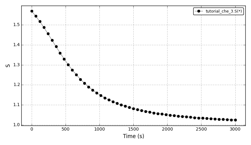
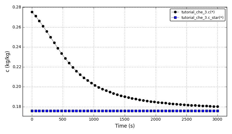
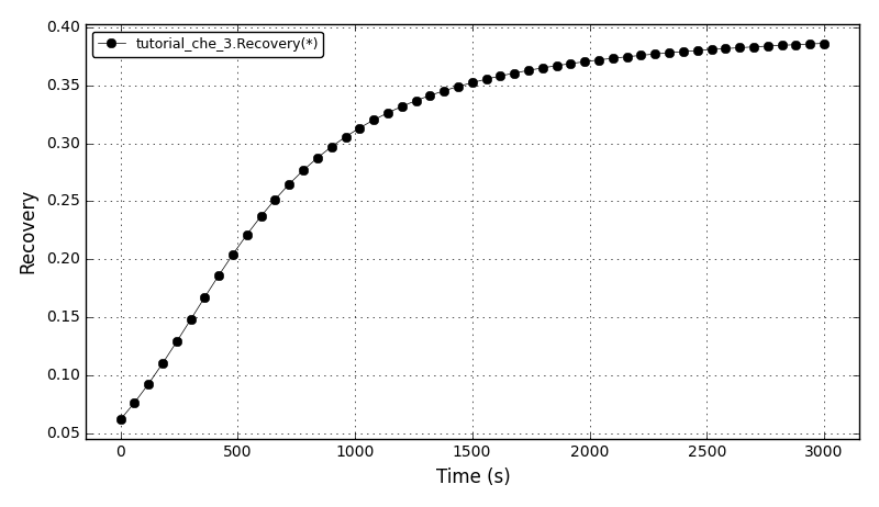
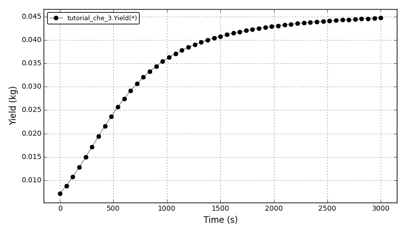
Batch reactor seeded crystallisation using the method of moments.

References (model equations and input parameters):

• Nikolic D.D., Frawley P.J. (2016) Application of the Lagrangian Meshfree Approach to Modelling of Batch Crystallisation: Part I - Modelling of Stirred Tank Hydrodynamics. Chemical Engineering Science 145:317-328. doi:10.1016/j.ces.2015.08.052

• Mitchell N.A., O’Ciardha C.T., Frawley P.J. (2011) Estimation of the growth kinetics for the cooling crystallisation of paracetamol and ethanol solutions. Journal of Crystal Growth 328:39-49. doi:10.1016/j.jcrysgro.2011.06.016

The main assumptions:

• Seeded crystallisation

• Ideal mixing

• Fixed cooling rate

• Size independent growth

Solubility of Paracetamol in ethanol:

---------------------------------------------------------
Temperature       Solubility          Solubility 
     C        kg Parac./kg EtOH   mol Parac./m3 EtOH
---------------------------------------------------------
      0           0.11362                593.0387
     10           0.14128                737.4215
     20           0.17568                916.9562
     30           0.21845                1140.2008
     40           0.27163                1417.7972
     50           0.33777                1762.9779
     60           0.42000                2192.1973
---------------------------------------------------------

The supersaturation plot:

The concentration plot:

The recovery plot:

The yield plot:

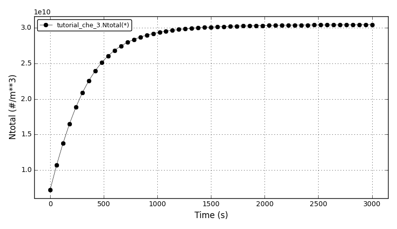
The total number of crystals plot:

Files

Model report	tutorial_che_3.xml
Runtime model report	tutorial_che_3-rt.xml
Source code	tutorial_che_3.py

Chem. Eng. Example 4

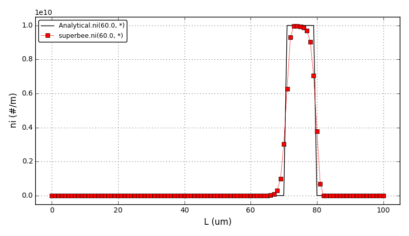
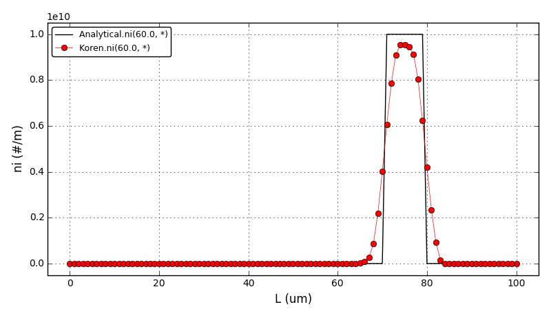
This example shows a comparison between the analytical results and the discretised population balance equations results solved using the cell centered finite volume method employing the high resolution upwind scheme (Van Leer k-interpolation with k = 1/3) and a range of flux limiters.

This tutorial can be run from the console only.

The problem is from the section 4.1.1 Size-independent growth I of the following article:

• Nikolic D.D., Frawley P.J. Application of the Lagrangian Meshfree Approach to Modelling of Batch Crystallisation: Part II – An Efficient Solution of Integrated CFD and Population Balance Equations. Preprints 2016, 20161100128. doi:10.20944/preprints201611.0012.v1

and also from the section 3.1 Size-independent growth of the following article:

• Qamar S., Elsner M.P., Angelov I.A., Warnecke G., Seidel-Morgenstern A. (2006) A comparative study of high resolution schemes for solving population balances in crystallization. Computers and Chemical Engineering 30(6-7):1119-1131. doi:10.1016/j.compchemeng.2006.02.012

The growth-only crystallisation process was considered with the constant growth rate of 1μm/s and the following initial number density function:

n(L,0): 1E10, if 10μm < L < 20μm
           0, otherwise

The crystal size in the range of [0, 100]μm was discretised into 100 elements. The analytical solution in this case is equal to the initial profile translated right in time by a distance Gt (the growth rate multiplied by the time elapsed in the process).

The flux limiters used in the model are:

• HCUS

• HQUICK

• Koren

• monotinized_central

• minmod

• Osher

• ospre

• smart

• superbee

• Sweby

• UMIST

• vanAlbada1

• vanAlbada2

• vanLeer

• vanLeer_minmod

Comparison of L1- and L2-norms (ni_HR - ni_analytical):

--------------------------------------
         Scheme  L1         L2
--------------------------------------
       superbee  1.786e+10  7.016e+09
          Sweby  2.817e+10  8.614e+09
          Koren  3.015e+10  9.293e+09
          smart  2.961e+10  9.326e+09
             MC  3.258e+10  9.807e+09
           HCUS  3.638e+10  1.001e+10
         HQUICK  3.622e+10  1.005e+10
  vanLeerMinmod  3.581e+10  1.011e+10
        vanLeer  3.874e+10  1.059e+10
          ospre  4.139e+10  1.094e+10
          UMIST  4.363e+10  1.136e+10
          Osher  4.579e+10  1.156e+10
     vanAlbada1  4.574e+10  1.157e+10
         minmod  5.653e+10  1.325e+10
     vanAlbada2  5.456e+10  1.331e+10
 -------------------------------------

The comparison of number density functions between the analytical solution and the solution obtained using high-resolution scheme with the Superbee flux limiter at t=60s:

The comparison of number density functions between the analytical solution and the solution obtained using high-resolution scheme with the Koren flux limiter at t=60s:

Animation:

Files

Source code	tutorial_che_4.py
Analytical solution	fl_analytical.py

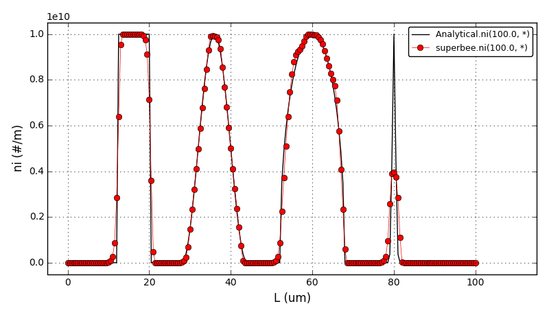
Chem. Eng. Example 5

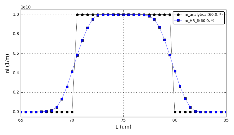
Similar to the chem. eng. example 4, this example shows a comparison between the analytical results and the discretised population balance equations results solved using the cell centered finite volume method employing the high resolution upwind scheme (Van Leer k-interpolation with k = 1/3) and a range of flux limiters.

This tutorial can be run from the console only.

The problem is from the section 4.1.2 Size-independent growth II of the following article:

• Nikolic D.D., Frawley P.J. Application of the Lagrangian Meshfree Approach to Modelling of Batch Crystallisation: Part II – An Efficient Solution of Integrated CFD and Population Balance Equations. Preprints 2016, 20161100128. doi:10.20944/preprints201611.0012.v1

and also from the section 3.2 Size-independent growth of the following article:

• Qamar S., Elsner M.P., Angelov I.A., Warnecke G., Seidel-Morgenstern A. (2006) A comparative study of high resolution schemes for solving population balances in crystallization. Computers and Chemical Engineering 30(6-7):1119-1131. doi:10.1016/j.compchemeng.2006.02.012

Again, the growth-only crystallisation process was considered with the constant growth rate of 0.1μm/s and with the different initial number density function:

n(L,0):                      0, if        L <= 2.0μm
                          1E10, if  2μm < L <= 10μm (region I)
                             0, if 10μm < L <= 18μm
      1E10*cos^2(pi*(L-26)/64), if 18μm < L <= 34μm (region II)
                             0, if 34μm < L <= 42μm
      1E10*sqrt(1-(L-50)^2/64), if 42μm < L <= 58μm (region III)
                             0, if 58μm < L <= 66μm
1E10*exp(-(L-70)^2/(2sigma^2)), if 66μm < L <= 74μm (region IV)
                             0, if 74μm < L

The crystal size in the range of [0, 100]μm was discretised into 200 elements. The analytical solution in this case is equal to the initial profile translated right in time by a distance Gt (the growth rate multiplied by the time elapsed in the process).

Comparison of L1- and L2-norms (ni_HR - ni_analytical):

-------------------------------------
        Scheme  L1         L2
-------------------------------------
      superbee  4.464e+10  1.015e+10
         smart  4.727e+10  1.120e+10
         Koren  4.861e+10  1.141e+10
         Sweby  5.435e+10  1.142e+10
            MC  5.129e+10  1.162e+10
        HQUICK  5.531e+10  1.194e+10
          HCUS  5.528e+10  1.194e+10
 vanLeerMinmod  5.600e+10  1.202e+10
       vanLeer  5.814e+10  1.225e+10
         ospre  6.131e+10  1.252e+10
         UMIST  6.181e+10  1.259e+10
         Osher  6.690e+10  1.275e+10
    vanAlbada1  6.600e+10  1.281e+10
        minmod  7.751e+10  1.360e+10
    vanAlbada2  7.901e+10  1.413e+10
-------------------------------------

The comparison of number density functions between the analytical solution and the solution obtained using high-resolution scheme with the Superbee flux limiter at t=100s:

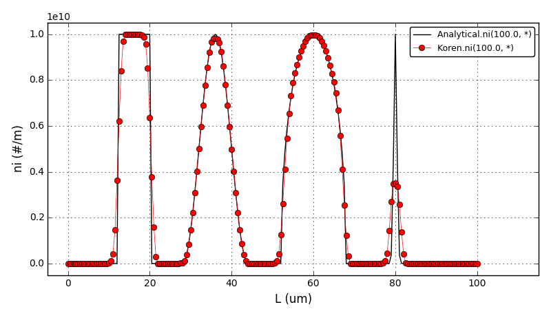
The comparison of number density functions between the analytical solution and the solution obtained using high-resolution scheme with the Koren flux limiter at t=100s:

Files

Source code	tutorial_che_5.py
Analytical solution	fl_analytical.py

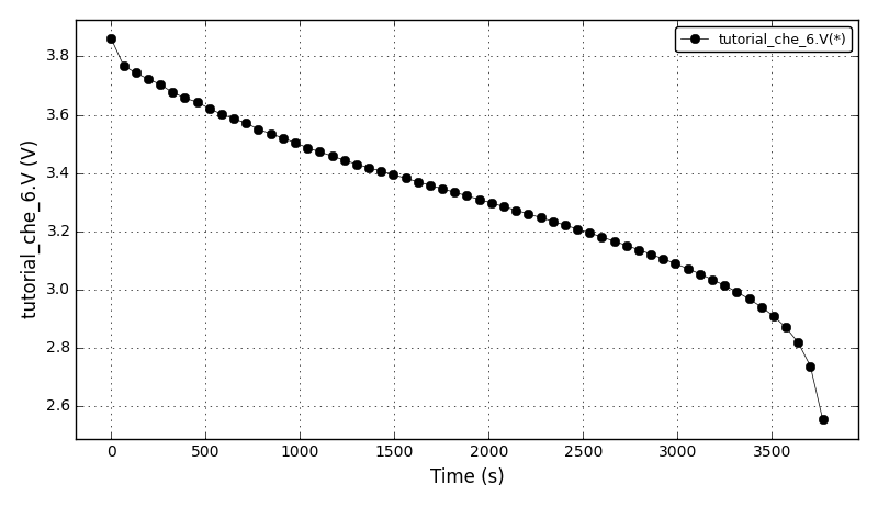
Chem. Eng. Example 6

Model of a lithium-ion battery based on porous electrode theory as developed by John Newman and coworkers. In particular, the equations here are based on a summary of the methodology by Karen E. Thomas, John Newman, and Robert M. Darling,

Thomas K., Newman J., Darling R. (2002). Mathematical Modeling of Lithium Batteries in Advances in Lithium-ion Batteries. Springer US. 345-392. doi:10.1007/0-306-47508-1_13

A few simplifications have been made rather than implementing the more complete model described there. For example, the following assumptions have (currently) been made:

• two porous electrodes are used rather than providing the option for a “half cell” in which one electrode is lithium foil.

• conductivity in the electron-conducting phase is infinite

• constant exchange current density in Butler-Volmer reaction expression

• no electrolyte convection

• constant and uniform solvent concentration (ions vary according to concentrated solution theory)

• monodisperse particles in electrode

• no volume occupied by binder, filler, etc. in the electrode

The up to date version of the model is available at Raymond’s GitHub repository: https://github.com/raybsmith/daetools-example-battery.

The voltage plot:

The current plot:

Files

Model report	tutorial_che_6.xml
Runtime model report	tutorial_che_6-rt.xml
Source code	tutorial_che_6.py

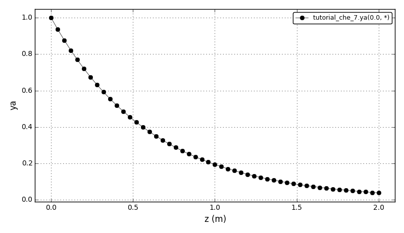
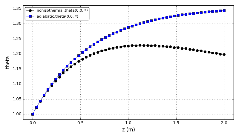
Chem. Eng. Example 7

Steady-state Plug Flow Reactor with energy balance and first order reaction:

A -> B

The problem is example 9.4.3 from the section 9.4 Nonisothermal Plug Flow Reactor from the following book:

• Davis M.E., Davis R.J. (2003) Fundamentals of Chemical Reaction Engineering. McGraw Hill, New York, US. ISBN 007245007X.

The dimensionless concentration plot:

The dimensionless temperature plot (adiabatic and nonisothermal cases):

Files

Model report	tutorial_che_7.xml
Runtime model report	tutorial_che_7-rt.xml
Source code	tutorial_che_7.py

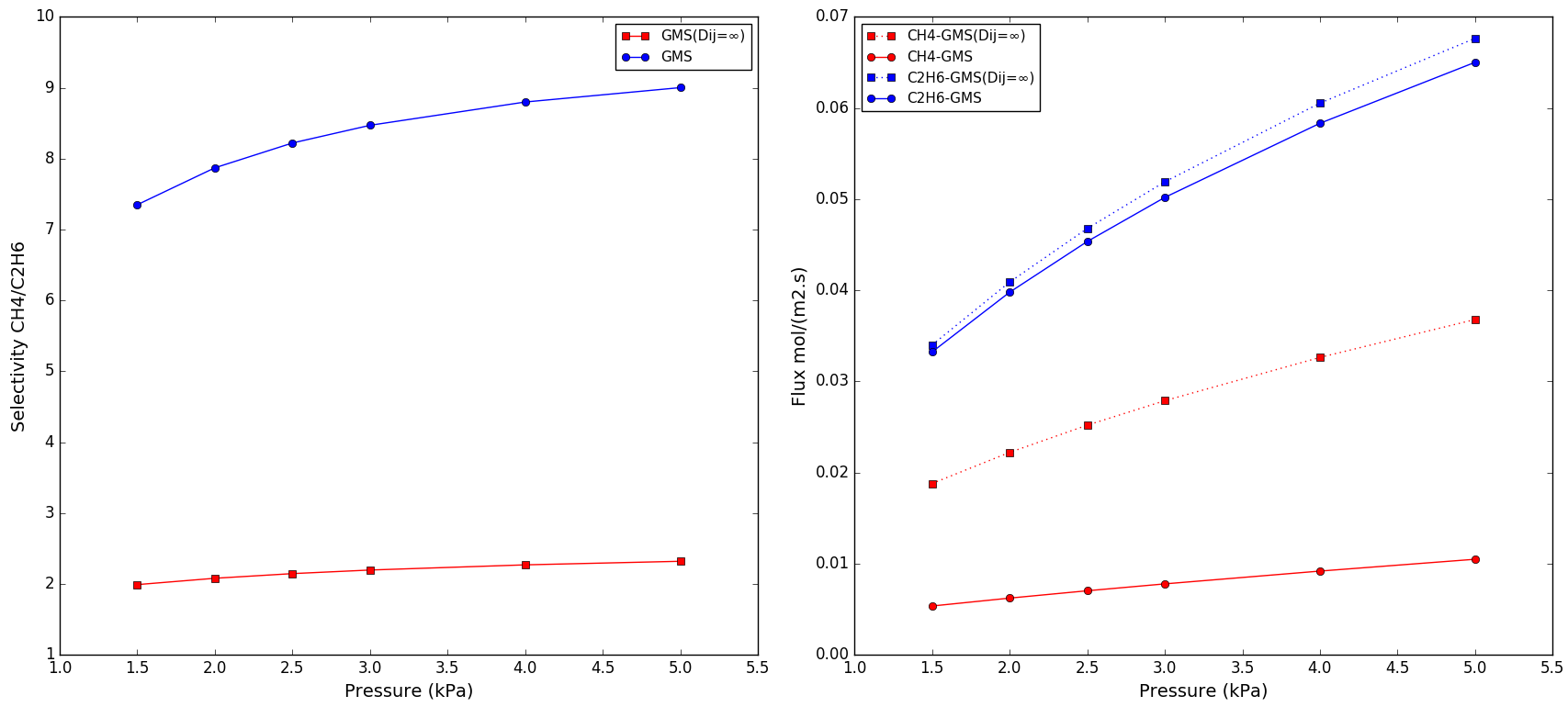
Chem. Eng. Example 8

Model of a gas separation on a porous membrane with a metal support. The model employs the Generalised Maxwell-Stefan (GMS) equations to predict fluxes and selectivities. The membrane unit model represents a generic two-dimensonal model of a porous membrane and consists of four models:

• Retentate compartment (isothermal axially dispersed plug flow)

• Micro-porous membrane

• Macro-porous support layer

• Permeate compartment (the same transport phenomena as in the retentate compartment)

The retentate compartment, the porous membrane, the support layer and the permeate compartment are coupled via molar flux, temperature, pressure and gas composition at the interfaces. The model is described in the section 2.2 Membrane modelling of the following article:

• Nikolic D.D., Kikkinides E.S. (2015) Modelling and optimization of PSA/Membrane separation processes. Adsorption 21(4):283-305. doi:10.1007/s10450-015-9670-z

and in the original Krishna article:

• Krishna R. (1993) A unified approach to the modeling of intraparticle diffusion in adsorption processes. Gas Sep. Purif. 7(2):91-104. doi:10.1016/0950-4214(93)85006-H

This version is somewhat simplified for it only offers an extended Langmuir isotherm. The Ideal Adsorption Solution theory (IAS) and the Real Adsorption Solution theory (RAS) described in the articles are not implemented here.

The problem modelled is separation of hydrocarbons (CH4+C2H6) mixture on a zeolite (silicalite-1) membrane with a metal support from the section ‘Binary mixture permeation’ of the following article:

• van de Graaf J.M., Kapteijn F., Moulijn J.A. (1999) Modeling Permeation of Binary Mixtures Through Zeolite Membranes. AIChE J. 45:497–511. doi:10.1002/aic.690450307

The CH4 and C2H6 fluxes, and CH4/C2H6 selectivity plots for two cases: GMS and GMS(Dij=∞), 1:1 mixture, and T = 303 K:

Files

Model report	tutorial_che_8.xml
Runtime model report	tutorial_che_8-rt.xml
Source code	tutorial_che_8.py
Membrane unit	membrane_unit.py
Variable types	membrane_variable_types.py
Membrane model	membrane.py
Support model	support.py
In/out compartment	compartment.py

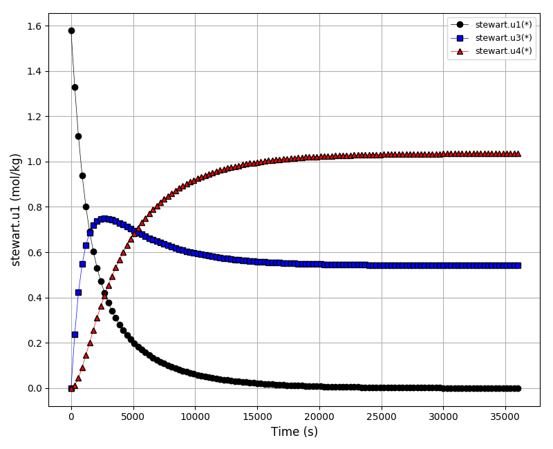
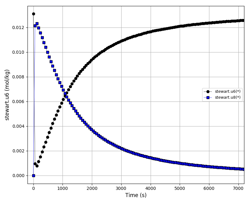
Chem. Eng. Example 9

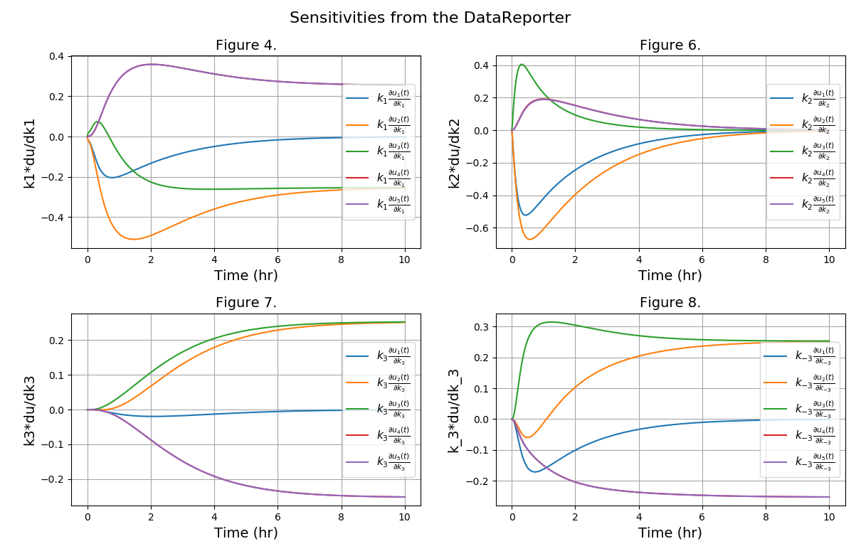
Chemical reaction network from the Dow Chemical Company described in the following article:

• Caracotsios M., Stewart W.E. (1985) Sensitivity analysis of initial value problems with mixed odes and algebraic equations. Computers & Chemical Engineering 9(4):359-365. doi:10.1016/0098-1354(85)85014-6

The sensitivity analysis is enabled and the sensitivity data can be obtained in two ways:

• Directly from the DAE solver in the user-defined Run function using the DAESolver.SensitivityMatrix property.

• From the data reporter as any ordinary variable.

The concentrations plot (u1, u3, u4):

The concentrations plot (u6, u8):

The sensitivities plot (k2*du1/dk2, k2*du2/dk2, k2*du3/dk2, k2*du4/dk2, k2*du5/dk2):

Files

Model report	tutorial_che_9.xml
Runtime model report	tutorial_che_9-rt.xml
Source code	tutorial_che_9.py

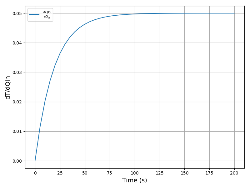
Sensitivity Analysis Example 1

This tutorial illustrates calculation of the sensitivity of the results with respect to the model parameters using forward sensitivity analysis method in DAE Tools.

This model has one state variable (T) and one degree of freedom (Qin). Qin is set as a parameter for sensitivity analysis.

The integration of sensitivities per specified parameters is enabled and the sensitivities can be reported to the data reporter like any ordinary variable by setting the boolean property simulation.ReportSensitivities to True.

Raw sensitivity matrices can be saved into a specified directory using the simulation.SensitivityDataDirectory property (before a call to Initialize). The sensitivity matrics are saved in .mmx coordinate format where the first dimensions is Nparameters and second Nvariables: S[Np, Nvars].

The plot of the sensitivity of T per Qin:

Files

Model report	tutorial_sa_1.xml
Runtime model report	tutorial_sa_1-rt.xml
Source code	tutorial_sa_1.py

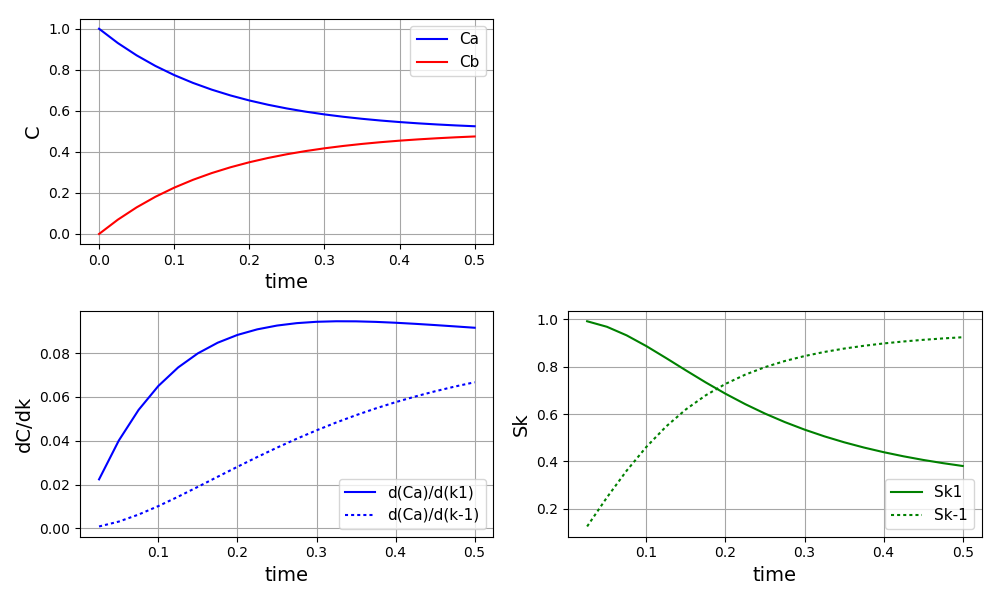
Sensitivity Analysis Example 2

This tutorial illustrates the local derivative-based sensitivity analysis method available in DAE Tools.

The problem is adopted from the section 2.1 of the following article:

• A. Saltelli, M. Ratto, S. Tarantola, F. Campolongo. Sensitivity Analysis for Chemical Models. Chem. Rev. (2005), 105(7):2811-2828. doi:10.1021/cr040659d

The model is very simple and describes a simple reversible chemical reaction A <-> B, with reaction rates k1 and k_1 for the direct and inverse reactions, respectively. The reaction rates are uncertain and are described by continuous random variables with known probability density functions. The standard deviation is 0.3 for k1 and 1 for k_1. The standard deviation of the concentration of the species A is approximated using the following expression defined in the article:

stddev(Ca)**2 = stddev(k1)**2 * (dCa/dk1)**2 + stddev(k_1)**2 * (dCa/dk_1)**2

The following derivative-based measures are used in the article:

• Derivatives dCa/dk1 and dCa/dk_1 calculated using the forward sensitivity method

• Sigma normalised derivatives:

  S(k1)  = stddev(k1) / stddev(Ca) * dCa/dk1
  S(k_1) = stddev(k_1)/ stddev(Ca) * dCa/dk_1
  

The plot of the concentrations, derivatives and sigma normalised derivatives:

Files

Model report	tutorial_sa_2.xml
Runtime model report	tutorial_sa_2-rt.xml
Source code	tutorial_sa_2.py

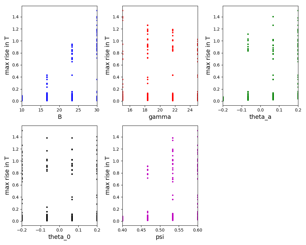
Sensitivity Analysis Example 3

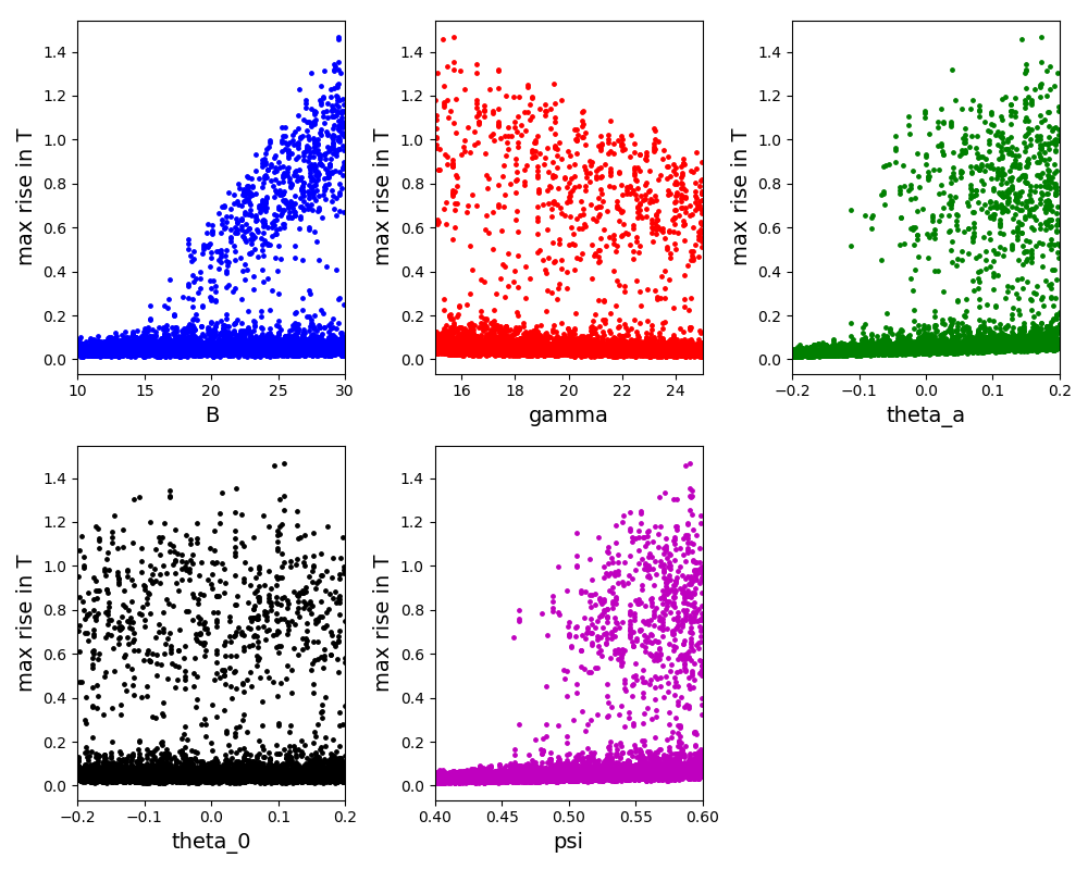
This tutorial illustrates the global variance-based sensitivity analysis methods available in the SALib python library.

The problem is adopted from the section 2.6 of the following article:

• A. Saltelli, M. Ratto, S. Tarantola, F. Campolongo. Sensitivity Analysis for Chemical Models. Chem. Rev. (2005), 105(7):2811-2828. doi:10.1021/cr040659d

The model describes a thermal analysis of a batch reactor, with exothermic reaction A -> B. The model equations are written in dimensionless form.

Three global sensitivity analysis methods available in SALib are applied:

• Morris (Elementary Effect/Screening method)

• Sobol (Variance-based methods)

• FAST (Variance-based methods)

Results from the sensitivity analysis:

-------------------------------------------------------
       Morris (N = 510)
-------------------------------------------------------
    Param          mu        mu*   mu*_conf      Sigma
        B    0.367412   0.367412   0.114161   0.546276
    gamma   -0.040556   0.056616   0.021330   0.111878
      psi    0.311563   0.311563   0.103515   0.504398
  theta_a    0.326932   0.326932   0.102303   0.490423
  theta_0    0.021208   0.023524   0.016015   0.074062
-------------------------------------------------------

-------------------------------------------------------
       Sobol (N = 6144)
-------------------------------------------------------
    Param          S1    S1_conf         ST    ST_conf
        B    0.094110   0.078918   0.581930   0.154737
    gamma   -0.002416   0.012178   0.044354   0.027352
      psi    0.171043   0.087782   0.524579   0.142115
  theta_a    0.072535   0.042848   0.523394   0.165736
  theta_0    0.002340   0.004848   0.008173   0.005956

Parameter pairs          S2    S2_conf
        B/gamma    0.180427   0.160979
          B/psi    0.260689   0.171367
      B/theta_a    0.143261   0.154060
      B/theta_0    0.177129   0.156582
      gamma/psi    0.000981   0.027443
  gamma/theta_a    0.004956   0.036554
  gamma/theta_0   -0.009392   0.027390
    psi/theta_a    0.166155   0.172727
    psi/theta_0   -0.016434   0.129177
theta_a/theta_0    0.109057   0.127287
-------------------------------------------------------

---------------------------------
       FAST (N = 6150)
---------------------------------
    Param          S1         ST
        B    0.135984   0.559389
    gamma    0.000429   0.029026
      psi    0.171291   0.602461
  theta_a    0.144617   0.534116
  theta_0    0.000248   0.040741
---------------------------------

The scatter plot for the Morris method:

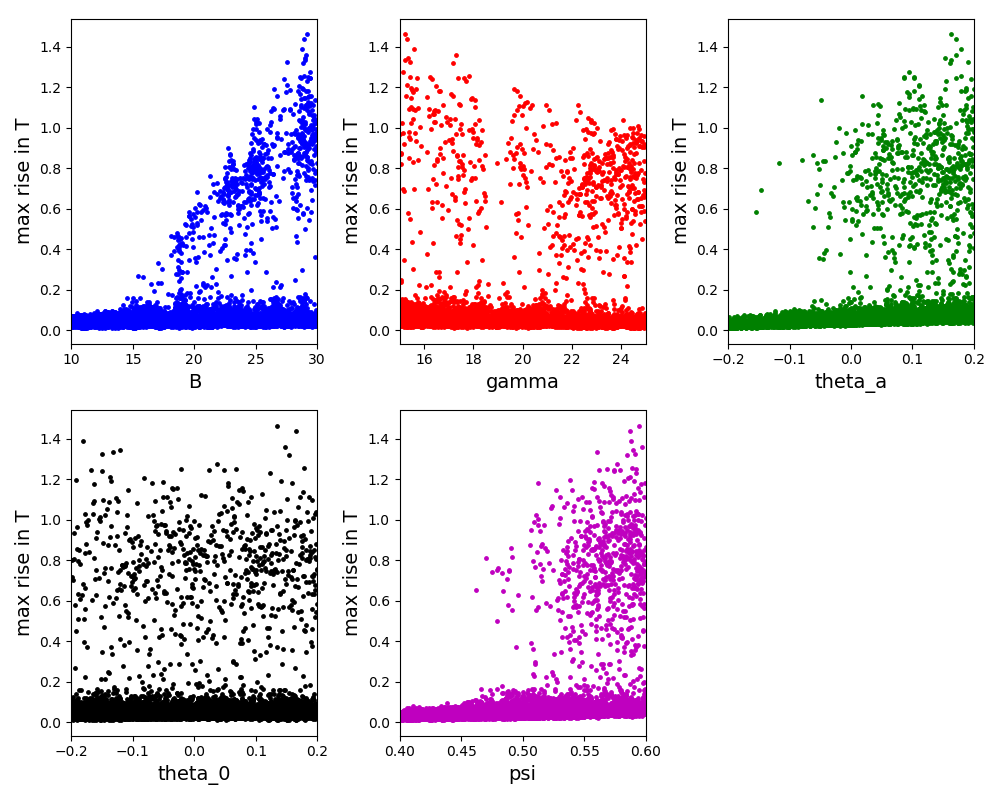
The scatter plot for the Sobol method:

The scatter plot for the FAST method:

Files

Model report	tutorial_sa_3.xml
Runtime model report	tutorial_sa_3-rt.xml
Source code	tutorial_sa_3.py

OpenCS Example DAE 1

Reimplementation of IDAS idasAkzoNob_dns example. The chemical kinetics problem with 6 non-linear diff. equations:

dy1_dt + 2*r1 - r2 + r3 + r4 = 0
dy2_dt + 0.5*r1 + r4 + 0.5*r5 - Fin = 0
dy3_dt - r1 + r2 - r3 = 0
dy4_dt + r2 - r3 + 2*r4 = 0
dy5_dt - r2 + r3 - r5 = 0
         Ks*y1*y4 - y6 = 0

where:

r1  = k1 * pow(y1,4) * sqrt(y2)
r2  = k2 * y3 * y4
r3  = k2/K * y1 * y5
r4  = k3 * y1 * y4 * y4
r5  = k4 * y6 * y6 * sqrt(y2)
Fin = klA * (pCO2/H - y2)

The system is stiff. The original results are in tutorial_opencs_dae_1.csv file.

Files

Source code	tutorial_opencs_dae_1.py
Auxiliary functions	tutorial_opencs_aux.py
DAE Tools model	tutorial_opencs_daetools_1.py
The original results	tutorial_opencs_dae_1.csv

OpenCS Example DAE 2

Reimplementation of DAE Tools tutorial1.py example. A simple heat conduction problem: conduction through a very thin, rectangular copper plate:

rho * cp * dT(x,y)/dt = k * [d2T(x,y)/dx2 + d2T(x,y)/dy2];  x in (0, Lx), y in (0, Ly)

Two-dimensional Cartesian grid (x,y) of 20 x 20 elements. The original results are in tutorial_opencs_dae_2.csv file.

Files

Source code	tutorial_opencs_dae_2.py
Auxiliary functions	tutorial_opencs_aux.py
The original results	tutorial_opencs_dae_2.csv

OpenCS Example DAE 3

Reimplementation of IDAS idasBruss_kry_bbd_p example. The PDE system is a two-species time-dependent PDE known as Brusselator PDE and models a chemically reacting system:

du/dt = eps1(d2u/dx2  + d2u/dy2) + u^2 v - (B+1)u + A
dv/dt = eps2(d2v/dx2  + d2v/dy2) - u^2 v + Bu

Boundary conditions: Homogenous Neumann. Initial Conditions:

u(x,y,t0) = u0(x,y) =  1  - 0.5*cos(pi*y/L)
v(x,y,t0) = v0(x,y) = 3.5 - 2.5*cos(pi*x/L)

The PDEs are discretized by central differencing on a uniform (Nx, Ny) grid. The model is described in:

• R. Serban and A. C. Hindmarsh. CVODES, the sensitivity-enabled ODE solver in SUNDIALS. In Proceedings of the 5th International Conference on Multibody Systems, Nonlinear Dynamics and Control, Long Beach, CA, 2005. ASME.

• M. R. Wittman. Testing of PVODE, a Parallel ODE Solver. Technical Report UCRL-ID-125562, LLNL, August 1996.

The original results are in tutorial_opencs_dae_3.csv file.

Files

Source code	tutorial_opencs_dae_3.py
Auxiliary functions	tutorial_opencs_aux.py
The original results	tutorial_opencs_dae_3.csv

OpenCS Example DAE 3 Groups

Reimplementation of tutorial_opencs_dae_3 using groups.

Files

Source code

tutorial_opencs_dae_3_groups.py

OpenCS Example DAE 3 Kernels

Reimplementation of tutorial_opencs_dae_3 using kernels.

Files

Source code

tutorial_opencs_dae_3_kernels.py

OpenCS Example DAE 3 Vector Kernels

Reimplementation of tutorial_opencs_dae_3 using auto- and explicitly-vectorised kernels.

Files

Source code

tutorial_opencs_dae_3_vector_kernels.py

OpenCS Example DAE 3 Fpga

Reimplementation of IDAS idasBruss_kry_bbd_p example. Simulated using the FPGA CSMachine (emulator version, at the moment). To run the example, Intel compiler must be setup by executing setvars.sh script:

source /opt/intel/oneapi/setvars.sh

Files

Source code

tutorial_opencs_dae_3_fpga.py

OpenCS Example DAE 3 Kernels FPGA

Reimplementation of tutorial_opencs_dae_3. Evaluated using FPGA evaluator (emulator version, at the moment). To run the example, Intel compiler must be setup by executing setvars.sh script:

source /opt/intel/oneapi/setvars.sh

Files

Source code

tutorial_opencs_dae_3_kernels_fpga.py

OpenCS Example DAE 3 Single Source

Reimplementation of tutorial_opencs_dae_3 using SYCL and Kokkos programming models.

Files

Source code

tutorial_opencs_dae_3_single_source.py

OpenCS Example DAE 5 CV

Code verification using the Method of Manufactured Solutions. It represents re-implementation of DAE Tools code verifications tutorial CV-2 - the 1-D transient convection-diffusion (Burger’s) equation. This example uses Dirichlet boundary conditions.

References:

1. G. Tryggvason. Method of Manufactured Solutions, Lecture 33: Predictivity-I, 2011. PDF

2. K. Salari and P. Knupp. Code Verification by the Method of Manufactured Solutions. SAND2000 – 1444 (2000). doi:10.2172/759450

3. P.J. Roache. Fundamentals of Verification and Validation. Hermosa, 2009. ISBN-10:0913478121

Note:

csSimulate cannot be called multiple times from python (multiple MPI init and finalize are not allowed). Therefore, the simulation are performed using the csSimulator binary (it has to be in the PATH for this to work).

Files

Source code

tutorial_opencs_dae_5_cv.py

OpenCS Example DAE 6 CV

Code verification using the Method of Manufactured Solutions. It represents re-implementation of DAE Tools code verifications tutorial CV-3 - the 1-D transient convection-diffusion (Burger’s) equation. This example uses Neumann boundary conditions.

References:

1. G. Tryggvason. Method of Manufactured Solutions, Lecture 33: Predictivity-I, 2011. PDF

2. K. Salari and P. Knupp. Code Verification by the Method of Manufactured Solutions. SAND2000 – 1444 (2000). doi:10.2172/759450

3. P.J. Roache. Fundamentals of Verification and Validation. Hermosa, 2009. ISBN-10:0913478121

Note:

csSimulate cannot be called multiple times from python (multiple MPI init and finalize are not allowed). Therefore, the simulation are performed using the csSimulator binary (it has to be in the PATH for this to work).

Files

Source code

tutorial_opencs_dae_6_cv.py

OpenCS Example DAE 7 CV

Code verification using the Method of Manufactured Solutions.

This problem and its solution in COMSOL Multiphysics <https://www.comsol.com> software is described in the COMSOL blog: Verify Simulations with the Method of Manufactured Solutions (2015), https://www.comsol.com/blogs/verify-simulations-with-the-method-of-manufactured-solutions.

Here, a 1D transient heat conduction problem in a bar of length L is solved using the Centered Finite Difference method:

dT/dt - k/(rho*cp) * d2T/dx2 = 0, x in [0,L]

Dirichlet boundary conditions are applied at both bar ends (500 K). Initial conditions are 500 K.

The manufactured solution is given by function u(x):

u(x) = 500 + (x/L) * (x/L - 1) * (t/tau)

Note:

csSimulate cannot be called multiple times from python (multiple MPI init and finalize are not allowed). Therefore, the simulation are performed using the csSimulator binary (it has to be in the PATH for this to work).

Files

Source code

tutorial_opencs_dae_7_cv.py

OpenCS Example DAE 8

In this example the Cahn-Hilliard equation is solved using the finite difference method. This equation describes the process of phase separation, where two components of a binary mixture separate and form domains pure in each component:

dc/dt = Diffusivity * nabla^2(mu)
mu = c^3 - c - gamma * nabla^2(c)

The mesh is a simple square (0-100)x(0-100). Input parameters are Diffusivity = 1 and gamma = 1. For both c an mu insulated boundary conditions are set (no flux on boundaries). Initial conditions are set to c(0) = 0.0 + c_noise where the noise is specified using the normal distribution with standard deviation of 0.1. The system is integrated for 500 seconds and the outputs are taken every 5 seconds.

Files

Source code

tutorial_opencs_dae_8.py

OpenCS Example DAE 8 Kernels

In this example the Cahn-Hilliard equation is solved using the finite difference method. This equation describes the process of phase separation, where two components of a binary mixture separate and form domains pure in each component:

dc/dt = Diffusivity * nabla^2(mu)
mu = c^3 - c - gamma * nabla^2(c)

The mesh is a simple square (0-100)x(0-100). Input parameters are Diffusivity = 1 and gamma = 1. For both c an mu insulated boundary conditions are set (no flux on boundaries). Initial conditions are set to c(0) = 0.0 + c_noise where the noise is specified using the normal distribution with standard deviation of 0.1. The system is integrated for 500 seconds and the outputs are taken every 5 seconds.

This version is implemented using kernels.

Files

Source code

tutorial_opencs_dae_8_kernels.py

OpenCS Example DAE 8 Vector Kernels

In this example the Cahn-Hilliard equation is solved using the finite difference method. This equation describes the process of phase separation, where two components of a binary mixture separate and form domains pure in each component:

dc/dt = Diffusivity * nabla^2(mu)
mu = c^3 - c - gamma * nabla^2(c)

The mesh is a simple square (0-100)x(0-100). Input parameters are Diffusivity = 1 and gamma = 1. For both c an mu insulated boundary conditions are set (no flux on boundaries). Initial conditions are set to c(0) = 0.0 + c_noise where the noise is specified using the normal distribution with standard deviation of 0.1. The system is integrated for 500 seconds and the outputs are taken every 5 seconds.

This version is implemented using auto- and explicitly vectorised kernels.

Files

Source code

tutorial_opencs_dae_8_vector_kernels.py

OpenCS Example DAE 9

Reimplementation of IDAS idasHeat2D_kry example. The DAE system solved is a spatial discretization of the PDE:

du/dt = d^2u/dx^2 + d^2u/dy^2

on the unit square. The boundary condition is u = 0 on all edges. Initial conditions are given by u = 16 x (1 - x) y (1 - y). The PDE is treated with central differences on a uniform M x M grid. The values of u at the interior points satisfy ODEs, and equations u = 0 at the boundaries are appended, to form a DAE system of size N = M^2. The grid size is 10 x 10.

Files

Source code

tutorial_opencs_dae_9.py

OpenCS Example ODE 1

Reimplementation of CVodes cvsRoberts_dns example. The Roberts chemical kinetics problem with 3 rate equations:

dy1/dt = -0.04*y1 + 1.e4*y2*y3
dy2/dt =  0.04*y1 - 1.e4*y2*y3 - 3.e7*(y2)^2
dy3/dt =  3.e7*(y2)^2

The problem is simulated for 4000 s, with the initial conditions:

y1 = 1.0
y2 = y3 = 0

The problem is stiff. The original results are in tutorial_opencs_ode_1.csv file.

Files

Source code	tutorial_opencs_ode_1.py
Auxiliary functions	tutorial_opencs_aux.py
The original results	tutorial_opencs_ode_1.csv

OpenCS Example ODE 2

Reimplementation of CVodes cvsAdvDiff_bnd example. The problem is simple advection-diffusion in 2-D:

du/dt = d2u/dx2 + 0.5 du/dx + d2u/dy2

on the rectangle:

0 <= x <= 2
0 <= y <= 1

and simulated for 1 s. Homogeneous Dirichlet boundary conditions are imposed, with the initial conditions:

u(x,y,t=0) = x(2-x)y(1-y)exp(5xy)

The PDE is discretized on a uniform Nx+2 by Ny+2 grid with central differencing. The boundary points are eliminated leaving an ODE system of size Nx*Ny. The original results are in tutorial_opencs_ode_2.csv file.

Files

Source code	tutorial_opencs_ode_2.py
Auxiliary functions	tutorial_opencs_aux.py
The original results	tutorial_opencs_ode_2.csv

OpenCS Example ODE 3

Reimplementation of CVodes cvsDiurnal_kry example. 2-species diurnal kinetics advection-diffusion PDE system in 2D:

dc(i)/dt = Kh*(d/dx)^2 c(i) + V*dc(i)/dx + (d/dy)(Kv(y)*dc(i)/dy) + Ri(c1,c2,t), i = 1,2

where:

R1(c1,c2,t) = -q1*c1*c3 - q2*c1*c2 + 2*q3(t)*c3 + q4(t)*c2
R2(c1,c2,t) =  q1*c1*c3 - q2*c1*c2 - q4(t)*c2
Kv(y) = Kv0*exp(y/5)

Kh, V, Kv0, q1, q2, and c3 are constants, and q3(t) and q4(t) vary diurnally. The problem is posed on the square:

0 <= x <= 20 (km)
30 <= y <= 50 (km)

with homogeneous Neumann boundary conditions, and integrated for 86400 sec (1 day). The PDE system is discretised using the central differences on a uniform 10 x 10 mesh. The original results are in tutorial_opencs_ode_3.csv file.

Files

Source code	tutorial_opencs_ode_3.py
Auxiliary functions	tutorial_opencs_aux.py
The original results	tutorial_opencs_ode_3.csv

OpenCS Example ODE 3 Groups

Reimplementation of tutorial_opencs_ode_3 using groups.

Files

Source code

tutorial_opencs_ode_3_groups.py

OpenCS Example ODE 3 Kernels

Reimplementation of tutorial_opencs_ode_3 using groups.

Files

Source code

tutorial_opencs_ode_3_kernels.py

The implementations of the COPS tests differ from the original ones in following:

• The Direct Sequential Approach has been applied while the original tests use the Direct Simultaneous Approach

• The analytical sensitivity Hessian matrix is not available. The limited memory Broyden–Fletcher–Goldfarb–Shanno (L-BFGS) algorithm from IPOPT is used.

As a consequence, the results slightly differ from the published results. In addition, the solver options should be tuned to achieve faster convergence.

Chem. Eng. Optimisation Example 1

Optimisation of the CSTR model and Van de Vusse reactions given in tutorial_che_1:

Not fully implemented yet.

Reference: G.A. Ridlehoover, R.C. Seagrave. Optimization of Van de Vusse Reaction Kinetics Using Semibatch Reactor Operation, Ind. Eng. Chem. Fundamen. 1973;12(4):444-447. doi:10.1021/i160048a700

Files

Model report	tutorial_che_opt_1.xml
Runtime model report	tutorial_che_opt_1-rt.xml
Source code	tutorial_che_opt_1.py

Chem. Eng. Optimisation Example 2

COPS test 5: Isomerization of α-pinene (parameter estimation of a dynamic system).

Very slow convergence.

Determine the reaction coefficients in the thermal isometrization of α-pinene (y1) to dipentene (y2) and allo-ocimen (y3) which in turn produces α- and β-pyronene (y4) and a dimer (y5).

Reference: Benchmarking Optimization Software with COPS 3.0, Mathematics and Computer Science Division, Argonne National Laboratory, Technical Report ANL/MCS-273, 2004. PDF

Experimental data taken from: Rocha A.M.A.C., Martins M.C., Costa M.F.P., Fernandes, E.M.G.P. (2016) Direct sequential based firefly algorithm for the α-pinene isomerization problem. 16th International Conference on Computational Science and Its Applications, ICCSA 2016, Beijing, China. doi:10.1007/978-3-319-42085-1_30

Run options:

• Simulation with optimal parameters: python tutorial_che_opt_2.py simulation

• Parameter estimation console run: python tutorial_che_opt_2.py console

• Parameter estimation GUI run: python tutorial_che_opt_2.py gui

Currently, the parameter estimation results are (solver options/scaling should be tuned):

Fobj  57.83097
p1    5.63514e-05
p2    2.89711e-05
p3    1.39979e-05
p4   18.67874e-05
p5    2.23770e-05

The concentration plots (for optimal ‘p’ from the literature):

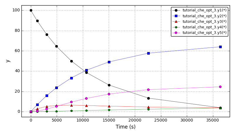
Files

Model report	tutorial_che_opt_2.xml
Runtime model report	tutorial_che_opt_2-rt.xml
Source code	tutorial_che_opt_2.py

Chem. Eng. Optimisation Example 3

COPS test 6: Marine Population Dynamics. (Not working properly)

Given estimates of the abundance of the population of a marine species at each stage (for example, nauplius, juvenile, adult) as a function of time, determine stage specific growth and mortality rates.

Reference: Benchmarking Optimization Software with COPS 3.0, Mathematics and Computer Science Division, Argonne National Laboratory, Technical Report ANL/MCS-273, 2004. PDF

Experimental data generated following the procedure described in the COPS test.

Run options:

• Simulation with optimal parameters: python tutorial_che_opt_3.py simulation

• Parameter estimation console run: python tutorial_che_opt_3.py console

• Parameter estimation GUI run: python tutorial_che_opt_3.py gui

Currently, the parameter estimation results are (suboptimal results obtained, solver options/scaling should be tuned):

Fobj =  1.920139e+8
m(0)    3.358765e-01
m(1)    4.711709e-01
m(2)    1.120524e-01
m(3)    8.509170e-02
m(4)    9.683579e-02
m(5)    1.919142e-01
m(6)    2.418778e-01
m(7)    2.421000e-01
g(0)    1.152995e+00
g(1)    7.529383e-01
g(2)    5.024174e-01
g(3)    5.704327e-01
g(4)    4.180333e-01
g(5)    3.185407e-01
g(6)    2.250250e-01

The distribution moments 1,2,5,6 plots (for optimal results from the literature):

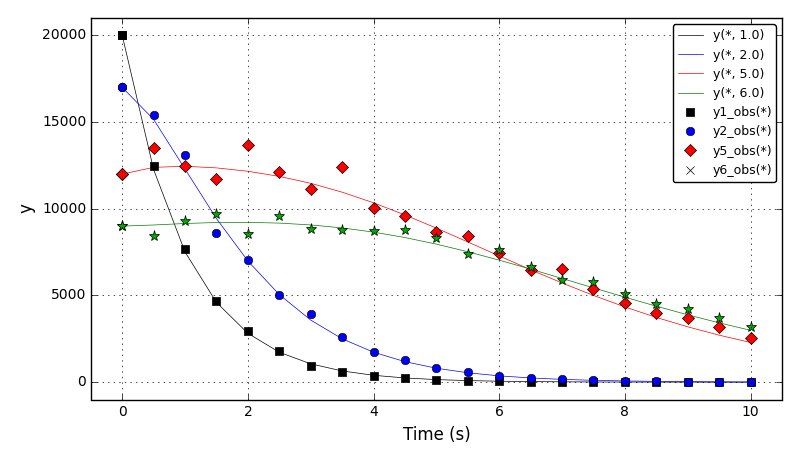
The distribution moments 3,4,7,8 plots (for optimal results from the literature):

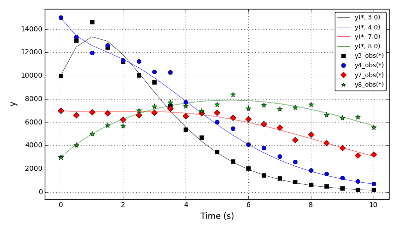
Files

Model report	tutorial_che_opt_3.xml
Runtime model report	tutorial_che_opt_3-rt.xml
Source code	tutorial_che_opt_3.py

Chem. Eng. Optimisation Example 4

COPS test 12: Catalytic Cracking of Gas Oil.

Determine the reaction coefficients for the catalytic cracking of gas oil into gas and other byproducts.

Reference: Benchmarking Optimization Software with COPS 3.0, Mathematics and Computer Science Division, Argonne National Laboratory, Technical Report ANL/MCS-273, 2004. PDF

Experimental data generated following the procedure described in the COPS test.

Run options:

• Simulation with optimal parameters: python tutorial_che_opt_4.py simulation

• Parameter estimation console run: python tutorial_che_opt_4.py console

• Parameter estimation GUI run: python tutorial_che_opt_4.py gui

Currently, the parameter estimation results are (solver options/scaling should be tuned):

Fobj = 4.841995e-3
p1   = 10.95289
p2   =  7.70601
p3   =  2.89625

The concentration plots (for optimal ‘p’ from the literature):

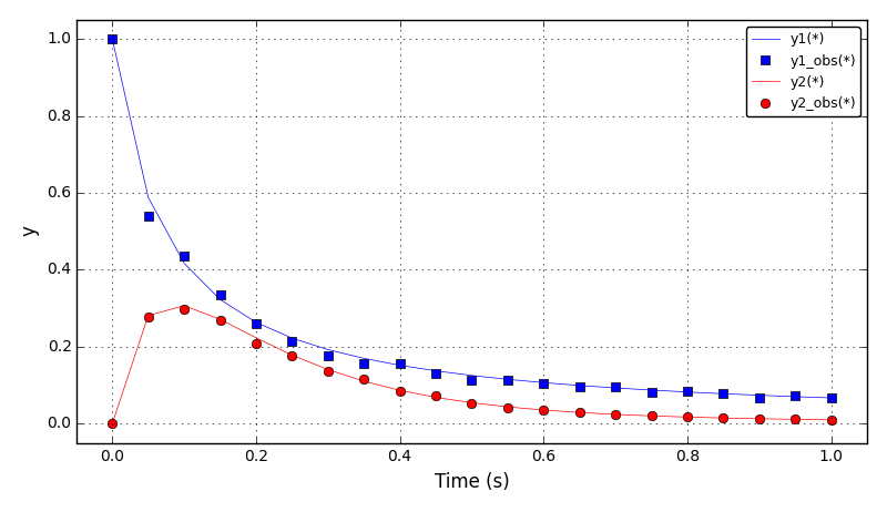
Files

Model report	tutorial_che_opt_4.xml
Runtime model report	tutorial_che_opt_4-rt.xml
Source code	tutorial_che_opt_4.py

Chem. Eng. Optimisation Example 5

COPS test 13: Methanol to Hydrocarbons.

Determine the reaction coefficients for the conversion of methanol into various hydrocarbons.

Reference: Benchmarking Optimization Software with COPS 3.0, Mathematics and Computer Science Division, Argonne National Laboratory, Technical Report ANL/MCS-273, 2004. PDF

Experimental data generated following the procedure described in the COPS test.

Run options:

• Simulation with optimal parameters: python tutorial_che_opt_5.py simulation

• Parameter estimation console run: python tutorial_che_opt_5.py console

• Parameter estimation GUI run: python tutorial_che_opt_5.py gui

Currently, the parameter estimation results are (solver options/scaling should be tuned):

Fobj = 1.274997e-2
p1 = 2.641769
p2 = 1.466245
p3 = 1.884254
p4 = 1.023885
p5 = 0.471067

The concentration plots (for optimal ‘p’ from the literature):

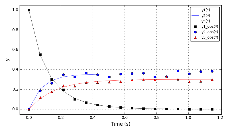
The concentration plots (for optimal ‘p’ from this optimisation):

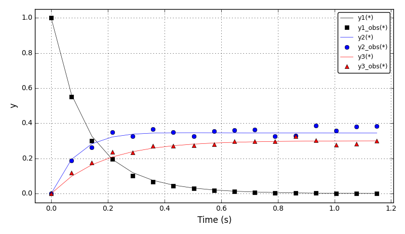
Files

Model report	tutorial_che_opt_5.xml
Runtime model report	tutorial_che_opt_5-rt.xml
Source code	tutorial_che_opt_5.py

Chem. Eng. Optimisation Example 6

COPS optimisation test 14: Catalyst Mixing.

Determine the optimal mixing policy of two catalysts along the length of a tubular plug flow reactor involving several reactions.

Reference: Benchmarking Optimization Software with COPS 3.0, Mathematics and Computer Science Division, Argonne National Laboratory, Technical Report ANL/MCS-273, 2004. PDF

In DAE Tools numerical solution of dynamic optimisation problems is obtained using the Direct Sequential Approach where, given a set of values for the decision variables, the system of ODEs are accurately integrated over the entire time interval using specific numerical integration formulae so that the objective functional can be evaluated. Therefore, the differential equations are satisfied at each iteration of the optimisation procedure.

In the COPS test, the problem is solved using the Direct Simultaneous Approach where the equations that result from a discretisation of an ODE model using orthogonal collocation on finite elements (OCFE), are incorporated directly into the optimisation problem, and the combined problem is then solved using a large-scale optimisation strategy.

The results: fobj = -4.79479E-2 (for Nh = 100) and -4.78676E-02 (for Nh = 200).

The control variables plot (for Nh = 100):

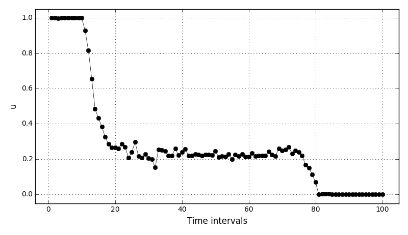
The control variables plot (for Nh = 200):

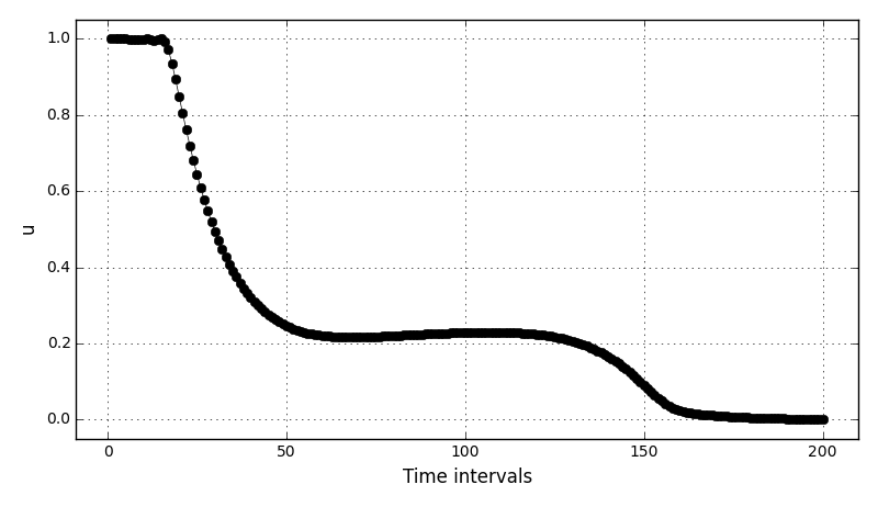
Files

Model report	tutorial_che_opt_6.xml
Runtime model report	tutorial_che_opt_6-rt.xml
Source code	tutorial_che_opt_6.py

Optimisation tutorial 1

This tutorial introduces IPOPT NLP solver, its setup and options.

Files

Model report	opt_tutorial1.xml
Runtime model report	opt_tutorial1-rt.xml
Source code	opt_tutorial1.py
C++ source code	opt_tutorial1.cpp

Optimisation tutorial 2

This tutorial introduces Bonmin MINLP solver, its setup and options.

Files

Model report	opt_tutorial2.xml
Runtime model report	opt_tutorial2-rt.xml
Source code	opt_tutorial2.py

Optimisation tutorial 3

This tutorial introduces NLOPT NLP solver, its setup and options.

Files

Model report	opt_tutorial3.xml
Runtime model report	opt_tutorial3-rt.xml
Source code	opt_tutorial3.py

Optimisation tutorial 4

This tutorial shows the interoperability between DAE Tools and 3rd party optimization software (scipy.optimize) used to minimize the Rosenbrock function.

DAE Tools simulation is used to calculate the objective function and its gradients, while scipy.optimize.fmin function (Nelder-Mead Simplex algorithm) to find the minimum of the Rosenbrock function.

Files

Model report	opt_tutorial4.xml
Runtime model report	opt_tutorial4-rt.xml
Source code	opt_tutorial4.py

Optimisation tutorial 5

This tutorial shows the interoperability between DAE Tools and 3rd party optimization software (scipy.optimize) used to fit the simple function with experimental data.

DAE Tools simulation object is used to calculate the objective function and its gradients, while scipy.optimize.leastsq function (a wrapper around MINPACK’s lmdif and lmder) implementing Levenberg-Marquardt algorithm is used to estimate the parameters.

Files

Model report	opt_tutorial5.xml
Runtime model report	opt_tutorial5-rt.xml
Source code	opt_tutorial5.py

Optimisation tutorial 6

daeMinpackLeastSq module test.

Files

Model report	opt_tutorial6.xml
Runtime model report	opt_tutorial6-rt.xml
Source code	opt_tutorial6.py

Optimisation tutorial 7

This tutorial introduces monitoring optimization progress.

Files

Model report	opt_tutorial7.xml
Runtime model report	opt_tutorial7-rt.xml
Source code	opt_tutorial7.py

What’s the time (C++)

Re-implementation of What’s the time? (AKA: Hello world!) example.

Source code: whats_the_time.cpp

Tutorial 1 (C++)

Re-implementation of Tutorial 1 example.

Source code: tutorial1.cpp

Tutorial 2 (C++)

Re-implementation of Tutorial 2 example.

Source code: tutorial2.cpp

Tutorial 4 (C++)

Re-implementation of Tutorial 4 example.

Source code: tutorial4.cpp

Tutorial 5 (C++)

Re-implementation of Tutorial 5 example.

Source code: tutorial5.cpp

Tutorial 6 (C++)

Re-implementation of Tutorial 6 example.

Source code: tutorial6.cpp

Tutorial 14 (C++)

Re-implementation of Tutorial 14 example.

Source code: tutorial14.cpp

Optimisation tutorial 1 (C++)

Re-implementation of Optimisation tutorial 1 example.

Source code: opt_tutorial1.cpp